Calculation 2: Phase line & Stability

Course subject(s) 1. Introducing Mathematical Modelling

Now that you can find equilibrium solutions of a differential equation, it is time to investigate what kinds of equilibrium solutions can occur. In the next video you will learn about this.

Note: in the video an example of an unstable equilibrium point is given. However, the definition of an unstable equilibrium point is not in the video. That you can find below, in the text.

Phase line & Stability of equilibrium points

Video

Other

Sorry, there don't seem to be any downloads..

Subtitles (captions) in other languages than provided can be viewed at YouTube. Select your language in the CC-button of YouTube.

Autonomous differential equations

In the video you have seen how you can construct a phase line from the direction field of a differential equation. You can only draw a phase line when the differential equation is a so-called autonomous differential equation.

In an autonomous differential equation, none of the terms depend explicitly on the independent variable.

In our differential equation,

the independent variable $t$ does not occur explicitly: although $P$ and $\frac{d P}{d t}$ are functions of $t$ , the time is not mentioned in the differential equation by itself. Our equation is autonomous.

A differential equation that is not autonomous is for example $\frac{d y}{d t} = 5 y (t) + \sin (t)$ . For this equation you cannot draw a phase line.

Different way to draw a phase line

Because our differential equation is autonomous, you can make a graph of $\frac{d P}{d t}$ versus $P (t)$ :

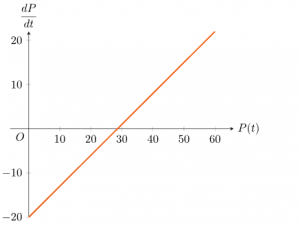
In this graph you can see that if $P (t)$ is smaller than the equilibrium value $\frac{20}{0.7}$ , the rate change, $\frac{d P}{d t}$ is negative, so the value of $P (t)$ will decrease. This means that in the phase line you should draw an arrow pointing in the decreasing direction for values below the equilibrium. This is the same as you have seen in the video. For values of $P (t)$ larger than the equilibrium, the value of $\frac{d P}{d t}$ is positive, so the arrow in this case must be pointing in the increasing direction.

Drawing a phase line vertical takes up a lot of room, so you could also draw the phase line horizontally. For the figure above, the phase line then becomes:

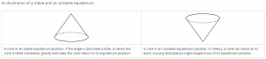
Stable equilibrium point

The equilibrium solution $P_{e} = \frac{20}{0.7}$ is an unstable equilibrium solution. For this we need a definition of what a stable equilibrium is.

We call an equilibrium point stable if any initial value close to the equilibrium point gives solutions that always remain close to the equilibrium point.

For many stable equilibrium points, the solutions that start close by, do not only remain close by, but for $t \to \infty$ the solutions even tend to the equilibrium point.

Unstable equilibrium point

Any equilibrium point which is not stable we call unstable, so there is at least one initial value close to the equilibrium which will give a solution that moves away from the equilibrium point.

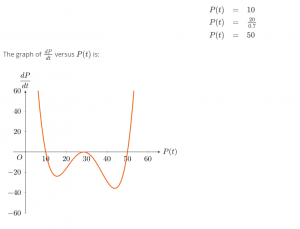
Another differential equation

In the next exercises we will consider a “slightly” different differential equation:

This differential equation has three equilibrium solutions:

Mathematical Modeling Basics by TU Delft OpenCourseWare is licensed under a Creative Commons Attribution-NonCommercial-ShareAlike 4.0 International License.
Based on a work at https://online-learning.tudelft.nl/courses/mathematical-modeling-basics/.