3.3.4 Worked example 3.2

Swinging pendulum

A child of mass $m$ is sitting on a swing with length $l$ . This can be seen as a pendulum, which for small $θ$ and in the absence of friction can be described by the following differential equation:

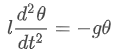
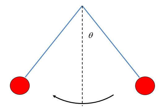
In the lecture it is explained that the solution for this differential equation is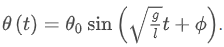

In this exercise we will focus on the motion of the pendulum and become familair with the solution of the differential equation

A different method

Maybe you came up with a different approach to determine the height. The swing can of course never be higher than its initial height. In the equilibrium position is considered to be zero height, the initial height can be calculated to be , which is shown below:

module 3 W.E. unit 2

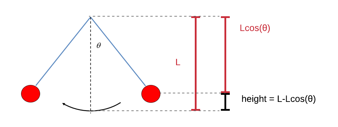
However, remember that the differential equation from the beginning only holds for small values of θ₀. The same holds for this answer! For small values of θ₀, both expressions for the maximum height are approximately equal to each other. This may seem strange, because the expression are very different, but it becomes clear when both functions are plotted together, as shown in the figure below:

module 3 W.E. unit 2

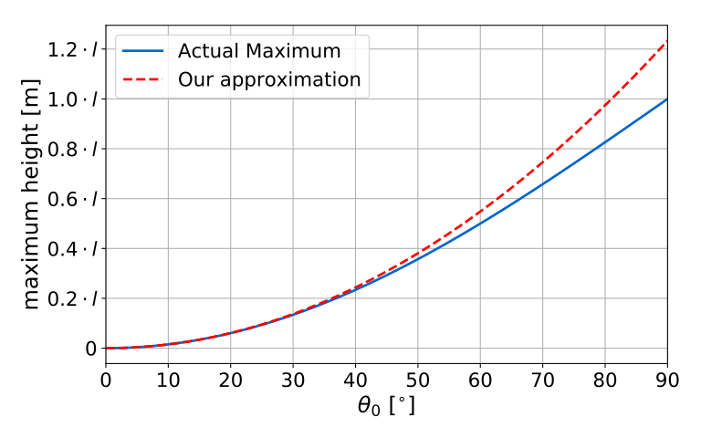
The real maximum is plotted in blue, and our approximation 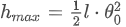is plotted in red. As you can see, both expression are almost equal if θ₀ is small. The reason for this is quite complicated and you do not have to worry about this. All of this will be explained in the first year of university!

Pre-University Physics by TU Delft OpenCourseWare is licensed under a Creative Commons Attribution-NonCommercial-ShareAlike 4.0 International License.
Based on a work at https://online-learning.tudelft.nl/courses/pre-university-physics/