On the previous page, you have learned to approximate solutions of a system of differential equations with Euler’s method. It is the same as for single differential equations, only now you work with a vector instead of a scalar. A graph of the solutions of the initial value problem is the following.

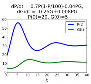
Both P and G have been plotted as functions of time t. Another way to visualise these solutions is to plot P and G against each other: to draw the solutions in the phase plane.

The phase plane is in this case the PG-plane. At any time t the solutions  P and G constitute a point (P(t),G(t)) in the phase plane. The collection of points (P(t),G(t)) for parameter t in an interval form a curve in the phase plane.

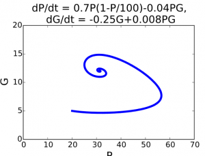
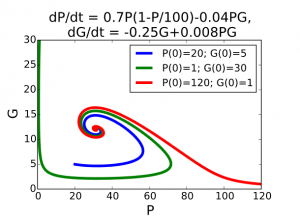
A solution curve drawn in the phase plane is called a trajectory. If you take another initial value for P and/or G, you obtain a different solution, and you can add its trajectory to the phase plane as well. A few trajectories in a phase plane constitute a phase portrait of the differential equations. An example of a phase portrait is the following graph: