


3.3 Calculation (linearisation)
Course subject(s)
3. Extending the model
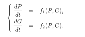
A mathematical model for interacting populations of rainbowfish (P(t)) and gourami (G(t)) in a 100-rainbowfish aquarium is the following system of differential equations.
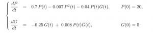
You have learned to simulate solutions with Euler’s method and to visualise these in the phase plane. Here you see a combination of trajectories, each with a different set of initial values.
Can we calculate some results analytically, so we can understand better how the parameters we have chosen for the model influence the results?
In this section you will learn how you to linearise the system in the neighbourhood of an equilibrium point. With the linearisations, you can predict some of the results analytically from the parameters.
The definition of an equilibrium point is:
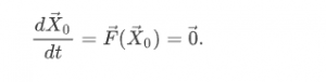
An equilibrium point of a system of differential equations
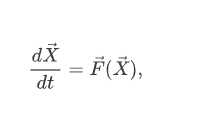
is a point X→0 where
You can see special things happening near the equilibrium points. For example near the point (100,0), you can see lines going first towards and then away from the equilibrium. Could we have predicted this behaviour using just the differential equations?
The answer is “Yes”, and in the remainder of this section you will learn how you can do this.
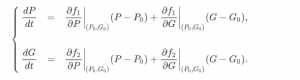
The first step in obtaining a prediction of the behavior near the equilibrium point is the linearisation of the differential equations around the equilibrium point.
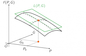
The linearisation of a function f(P,G) of two variables P and G is the process of approximating this function f in the neighbourhood of the point (P0,G0) by a function L(P,G) with the formula:
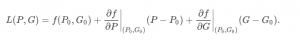
is the plane tangent to f in the point (P0,G0,f(P0,G0)). A visualisation of such a tangent plane is:
In our case we have two differential equations, and two functions to linearise. In a general form:

Mathematical Modeling Basics by TU Delft OpenCourseWare is licensed under a Creative Commons Attribution-NonCommercial-ShareAlike 4.0 International License.
Based on a work at https://online-learning.tudelft.nl/courses/mathematical-modeling-basics/.