


3.3 Calculation (saddle points and nodes)
Course subject(s)
3. Extending the model
Calculation (saddle points and nodes)
On the last page, some new notation was introduced:
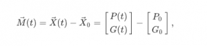
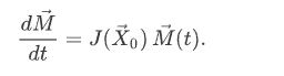
where (P0,G0) is an equilibrium point. You have learned that a system of differential equations that is linearised around an equilibrium point, can be written as:
When our rainbowfish/gourami system is linearised around (P0,G0)=(100,0), the result is:
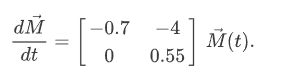
In the next video, Dennis explains what this new differential equation can tell you about the original differential equations.
Equilibrium points in a system

 Subtitles
Sorry, there don't seem to be any downloads..
Subtitles (captions) in other languages than provided can be viewed at YouTube. Select your language in the CC-button of YouTube.
In the video you have seen that (100,0) is a saddle point by looking at the solutions of the linearised differential equation. The behaviour of solutions near a saddle point is explained by the eigenvalues of the Jacobian matrix: one is positive, and one is negative.
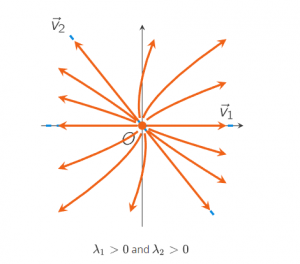
Of course, the eigenvalues of a 2×2-matrix can also be both negative or both positive. Then both factors eλ1t and eλ2t will either both decrease in time (when λ1<0 and λ2<0) or both increase in time, (when λ1>0 and λ2>0). The equilibrium points are then called nodes.
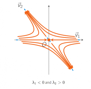
An equilibrium point X→0 is called a saddle point if the Jacobian matrix J(X→0) has one negative and one positive eigenvalue. A saddle point is unstable because some of the solutions that start near the equilibrium point (here the origin) leave the neighborhood of the origin. A typical sketch of the solutions near a saddle point in the phase plane is given by
An equilibrium point X→0 is called a stable node if the Jacobian matrix J(X→0) has two negative eigenvalues: all solutions that start near the equilibrium point stay near the equilirium point. An example of a phase portrait is
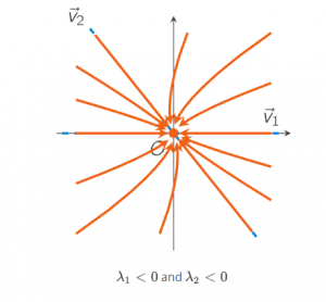
An equilibrium point X→0 is called an unstable node if the Jacobian matrix J(X→0) has two positive eigenvalues. A typical sketch of the solutions near an unstable node in the phase plane is given by

Mathematical Modeling Basics by TU Delft OpenCourseWare is licensed under a Creative Commons Attribution-NonCommercial-ShareAlike 4.0 International License.
Based on a work at https://online-learning.tudelft.nl/courses/mathematical-modeling-basics/.