


3.3 Calculation (spiral points)
Course subject(s)
3. Extending the model
On the previous page you learned about saddle points, stable nodes and unstable nodes. On this page you will encounter even more types of equilibrium points.
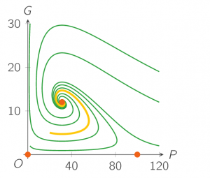
As you have seen in the last exercise, the eigenvalues of the Jacobian matrix in the point (31.25,12.03) are complex. Complex numbers are not positive or negative, so this equilibrium point is neither a stable node, nor an unstable node nor a saddle point. So what is it then?
the solutions for
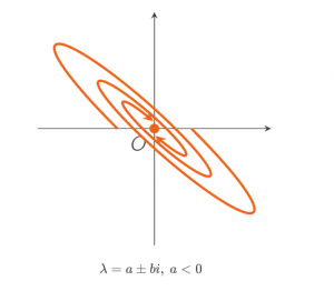
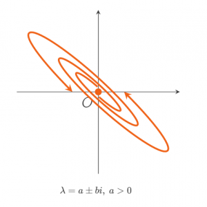
An equilibrium point ![]() is called a stable spiral point if the Jacobian matrix
is called a stable spiral point if the Jacobian matrix ![]() has two complex eigenvalues
has two complex eigenvalues ![]() with negative real parts: a<0. A typical sketch of the solutions near a stable spiral point in the phase plane is given by
with negative real parts: a<0. A typical sketch of the solutions near a stable spiral point in the phase plane is given by
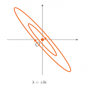
When a=0, the solution does not spiral inwards nor outwards, so the solution will be periodic, and in phase space the trajectory is a closed curve. Even though that curve is most often an ellips, the equilibrium point is called a circle point.
An equilibrium point ![]() is called a circle point if the Jacobian matrix
is called a circle point if the Jacobian matrix ![]() has two complex eigenvalues with zero real parts:
has two complex eigenvalues with zero real parts: ![]() .
.
Besides the six types of stability for equilibrium points discussed here, other types of stability exist, but these transcend the scope of this course.

Mathematical Modeling Basics by TU Delft OpenCourseWare is licensed under a Creative Commons Attribution-NonCommercial-ShareAlike 4.0 International License.
Based on a work at https://online-learning.tudelft.nl/courses/mathematical-modeling-basics/.