


3.3 Summary
Course subject(s)
3. Least Squares Estimation (LSE)
Geometry of least squares
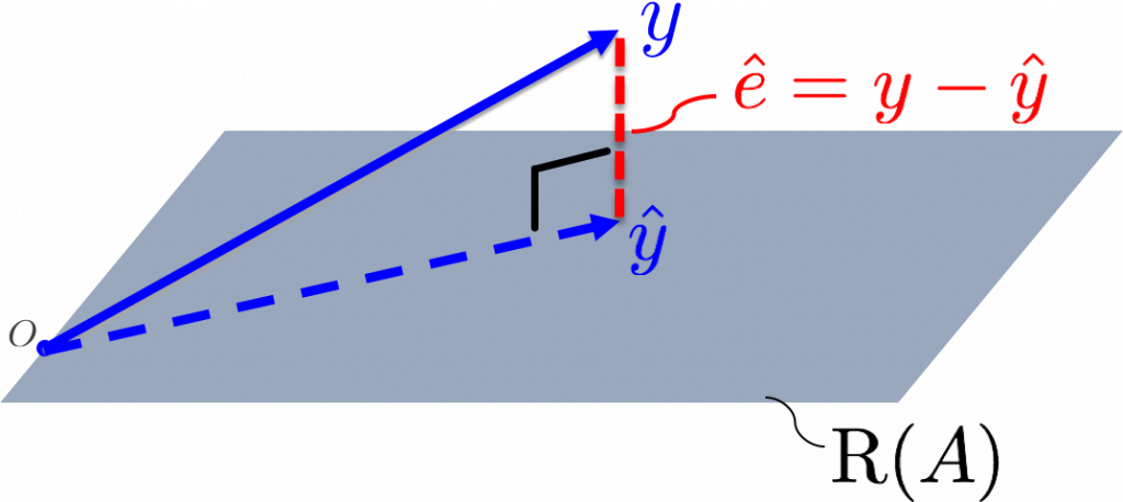
A geometric interpretation of least-squares can be given based on the figure below.
The system of observation equations, which is given by:
\[ y = Ax\]
is generally inconsistent. This means that we cannot find a solution for \(x\) such that the equality holds for a given observation vector.
In other words, the observation vector \(y\) is not in the range space of \(A\): \(y\notin \mathrm{R}(A)\), as shown in the figure. The grey plane depicts the range space \(\mathrm{R}(A)\), and \(y\) is outside this plane.
In order to make the model consistent, we introduced the error vector \(e\). Adding this error vector to the right-hand side of the equation, we can always find a solution for \(x\) and \(e\) (we now use the notation with hat to indicate a specific solution, or estimate):
\[ y = A\hat{x}+\hat{e}=\hat{y}+\hat{e}\]
Hence \(\hat{y}\) is in the range space of \(A\) (see figure), and \(\hat{e}\) is the residual vector that we need to add to \(\hat{y}\) in order to arrive back at \(y\).
The least-squares solution minimizes the squared sum of residuals, i.e. \(\hat{e}^T\hat{e}= \|\hat{e}\|^2\). This means that actually the length of the vector \(\hat{e}\) is minimized. And looking again at the figure this makes sense: it turns out that \(\hat{y}\) is the orthogonal projection of \(y\) on the range space of \(A\). This means that
\[\hat{e}\perp \mathrm{R}(A)\]
which is true if
\[A^T\hat{e} = 0 \]
If we work this out, we get:
\[\begin{align} A^T(y-\hat{y} ) &= 0 \\A^T(y-A\hat{x} ) &= 0\\A^Ty&= A^T A\hat{x}\end{align}\]
These are the so-called normal equations, from which we can see that
\[ \hat{x} =( A^T A)^{-1} A^T y\]
The least-squares solution! For \(\hat{y}\) we have:
\[ \hat{y} = A\hat{x} = A(A^TA)^{-1}A^T y= P_A y \]
where we introduced the orthogonal projector, which projects orthogonally on \(\mathrm{R}(A)\):
\[P_A = A(A^TA)^{-1}A^T\]
and indeed we showed that the least-squares solution \(\hat{y}\) is the orthogonal projection of \(y\) on the range space of \(A\).

Observation Theory: Estimating the Unknown by TU Delft OpenCourseWare is licensed under a Creative Commons Attribution-NonCommercial-ShareAlike 4.0 International License.
Based on a work at https://ocw.tudelft.nl/courses/observation-theory-estimating-unknown.