


3.4.1 to 3.4.5
Course subject(s)
3. Real Time Traffic Control

3.4.1 Requirements
This section describes which requirements for infracapacity can be derived from both the timetabling process and real time traffic management. And, the other way round, describes how infracapacity is a constraint for timetable development and the possibilities for real time rescheduling.
Long term scenarios: Requirements for infracapacity
The goal of infracapacity is to make sure that the prescribed timetable is executable. The timetable is based on the requirements for the desired passenger flows. This gives a certain train frequency on different parts of the railway network. The infrastructure should be able to handle the required amount of trains.
Real time traffic management (RTTM) ensures that a certain amount of trains remain operational during (unexpected) events. This is mostly done by applying predefined solutions. The disruptions mean that a part of the network is closed off and trains need to be able to divert other tracks/routes. The rail infrastructure needs to enable this when necessary, for instance by adding switches and buffer stations.
Short term scenarios: Requirements from infracapacity
The previous section shows timetabling and RTTM giving requirements to infra capacity. This shows where infrastructure should be improved or adjusted. This is only done for long term scenarios as changing the available infrastructure takes time and is often expensive so only suitable for large improvements in the system.
Another point of view is to see infracapacity as the starting point for timetabling and RTTM. There is a certain infrastructure available to use and timetabling and RTTM are designed based on this availability. This way of thinking is often applied for short term designs.
Requirements for timetable / RTTM: the available infrastructure is given. Use this to design your plan.
Requirements for the asset layer: make sure that the assets function on the established infrastructure network.
3.4.2 Theory vs Practice
A differentiation can be made between theoretical and practical infra capacity.
The theoretical capacity of a track can be defined as the number of trains that can be processed by a given infrastructure within a certain timeframe. This is determined by the travel time of trains and follow-up time between trains, which depend on the layout of the civil infrastructure, railway electric traction, safety margins and placement of security systems and block configurations.
The theoretical capacity cannot be obtained in reality due to limits within the actual situation, based on for example the availability, the types and the order of trains. In addition, other factors have to be taken into account like the behaviour of the driver, control systems and a buffer in the system for stable execution of the timetabling.
The components described above relate to the activities of the train operating company and partly to the traffic management systems. These systems affect how much of the theoretical capacity can be achieved during the execution of the timetable.
Balancing the use of capacity
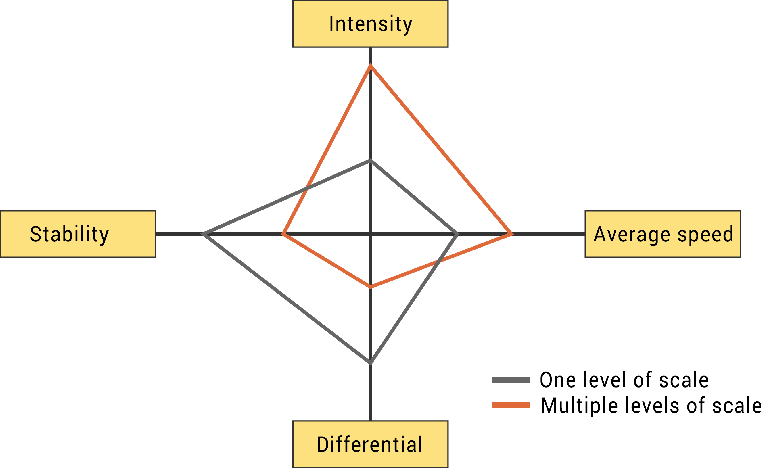
The balance between intensity and quality is an important steering parameter for the utilization of infrastructure. Intensity refers to the maximum amount of train services that can be delivered per hour. Quality refers to three main aspects: differentiation, average speed and the stability. Differentiation means the amount of levels of scale that are used. A large differentiation means that there are many different trains traveling at different speeds on the same track. A low differentiation means that there is only one type of train on the tracks. Average speed relates to the flow of the trains. The stability refers to the sensitivity to disturbances and can be expressed as the speed in which a disruption naturally dampens.
The utilization of infrastructure is a consideration between the intensity and the three quality aspects. The result of this process can be seen as a balance between these four utilization aspects. The balance between the four aspects can be illustrated by a diagram. The four different aspects form the axes. The utilization is given by a point on each axis. The capacity is represented by drawing a line through the points on the four axes. The resulting shape represents the available capacity. Because the utilization aspects are in balance, changing one point on an axis also affect one or more points on the other axes. The maximum theoretical intensity occurs when the three quality aspects are all zero.
The figure below illustrates the diagram and shows two examples of utilization profiles for rail infrastructure. For a train system with multiple levels of scale, the differentiation is large. Due to the faster trains on this network a large average speed is desired. This leads to relatively low intensities, for instance 4 to 6 train services per hour. A train system with one level of scale has low differentiation. The required average speed is relatively low so the intensity can become high, as much as 40 train services per hour.
3.4.3 High Frequent Routes
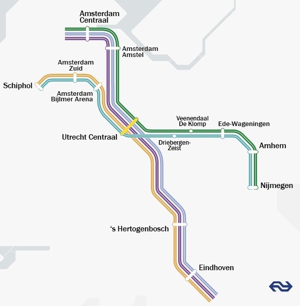
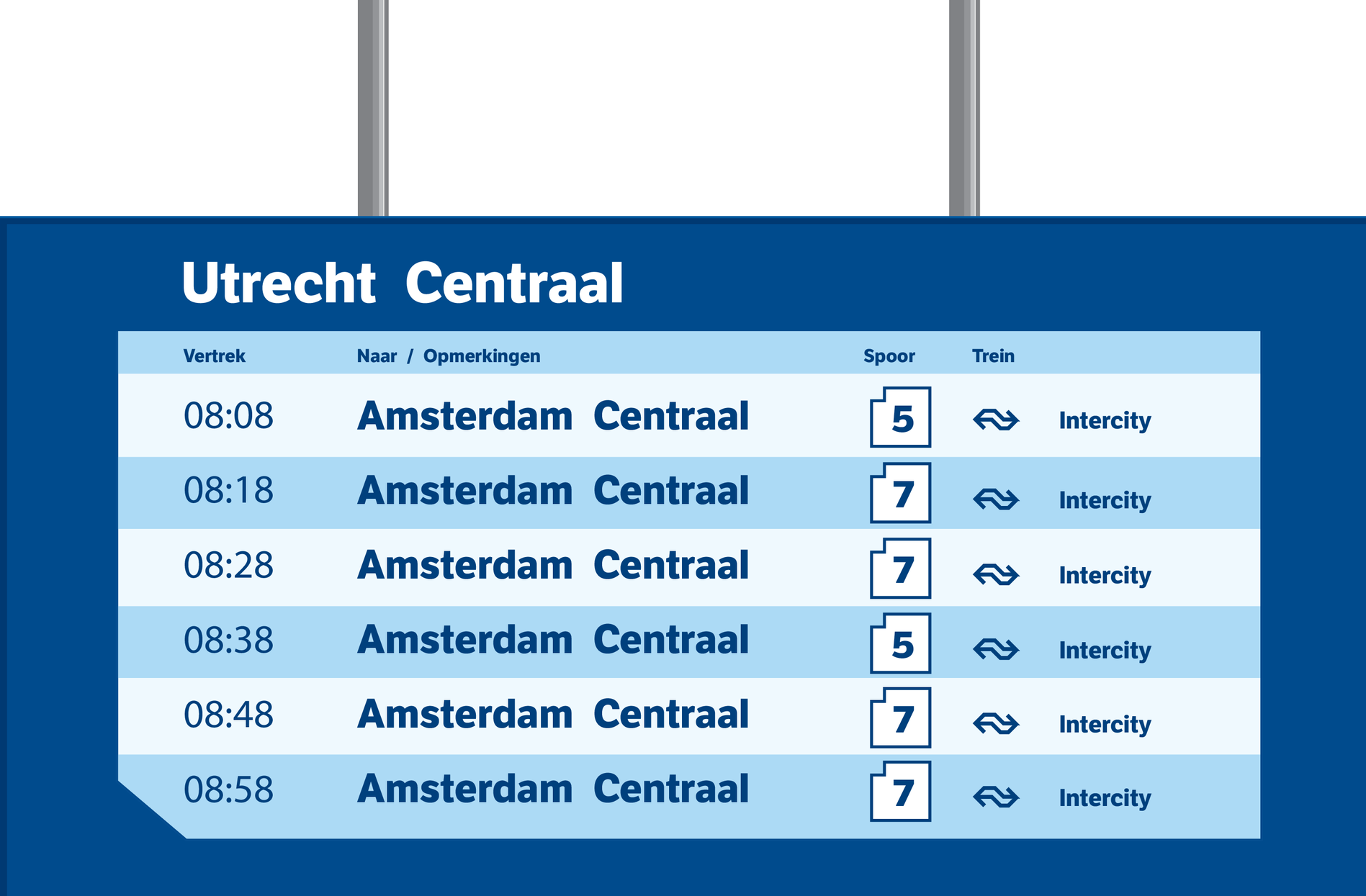
In the figure below, each line represents two intercity trains per hour in both directions in addition to the regular schedule of local trains. This means the connection between Amsterdam and Utrecht (two main railway stations in The Netherlands) is upgraded to a direct train every 10 minutes. The same goes for the connection between Utrecht and ‘s Hertogenbosch and Eindhoven (the two main cities in the south of the country).
Timetabling NS 2018 (source: NS – SpoorPro 2016)
The idea is that people don’t have to check the timetable and have an average waiting time of 5 minutes. If you go to the station without checking the schedule before, you might arrive right on time (waiting 1 minute) or you could have just missed the train (waiting 9 minutes). The gap between consistent train frequency divided by 2 is the average time people have to wait.
3.4.4 Signalling Systems: History
We will sum-up the different ways of signalling systems in a historical order to give you an idea of the development over the years. In our advanced course on Railway Operations we will go more into depth on this matter. The list ends with ERTMS (European Railway Traffic Management System). In the following section we will look at this new way of safety system in more detail.
Human based
At stations or at the beginning of each section of a line.
Hand signals or coloured flags by day and oil lamps by night.
No knowledge about the train’s location when out of sight.
Fixed signals
Many forms operated by signalmen with time interval working.
Early fixed signals were turnable boards on tall posts.
– Signal visible: stop; signal practically invisible: proceed
Disc and crossbar signal showed positive proceed aspects.
– Either the disc (indicating proceed) or crossbar (meaning stop) is visible
From 1841 on the semaphore signal was introduced.
Signal boxes:Centralizing the control of points and signals
Levers were connected to signals by wires and to points with rods.
One signalman (signaller) could operate all levers from a signal box.
In the early days signals were located on the roof of the signal box.
Later the signals were located at their correct positions.
Absolute Block system: Telegraph communication between signal boxes
Telegraph wires (1837) allowed communication between signal boxes.
Aim: to prevent more than one train in a block between signal boxes.
Block Instrument at neighbouring signal boxes showed:
– Line Blocked (white)
– Line Clear (green)
– Train On Line (red)
Absolute Block operation:
– Adjacent signallers communicated about the trains send and received over the line
– Signallers checked whether the trains arrived completely (observing tail lamp or flag)
Interlocking: Safe control of points and signals
From 1860 the levers were mechanically interlocked in a lever frame such that levers could only be pulled in a safe sequence.
From the end of 19th century the Block Instruments were also integrated in the signal interlocking such that signals could only be cleared when the block is at Line Clear.
The signaller still had to observe the tail lamps of arriving trains and operate points, signals, and Block Instruments to Line Blocked.
Early 20th century the levers were replaced by miniature levers operated by electric or pneumatic drives requiring less space and manpower.
Automatic block systems: Automatic train detection by track circuits
In the late 19th century the track circuit was developed:
– Electrical circuits in the rails could detect safely the absence of a train
From the 1920s track circuits were installed over entire blocks enabling automatic operation of signals
Automatic Block systems with connected successive signals:
– When a train passed a signal it changed to Danger
– The signal returned to Proceed when the train passed the next signal
Distant signals: Announcing main signals at danger
With increasing train speeds distant signals were introduced.
Distant signals were located more than the braking distance from the main signal.
If the main signal shows Danger the distant signal shows Caution, indicating that the train must brake.
With automatic blocks the block lengths were decreased and the main signal and distant signal (for the next signal) were combined.
Automatic train protection (ATP): Guard against driver errors
Train devices that warn or supervise and intervene when driver does not follow orders from trackside signals.
Relay interlockings: Routes setting with panel control
From the 1920s electric relay interlockings were developed.
This replaced lever operation by panel operation with route setting.
In addition, electric point machines allowed control over larger areas.
Panel operation enabled remote control over larger areas.
Electronic interlockings: Interlocking by software (since 1980)
Also known as processor-based and computer-based interlocking.
Track layouts displayed on monitors.
Points and signals interlocked by software and operated on console.
Centralized Traffic Control (CTC) over large areas possible.
ERTMS: Migration to interoperable signalling (future EU)
3.4.5 Signalling Systems: ERTMS
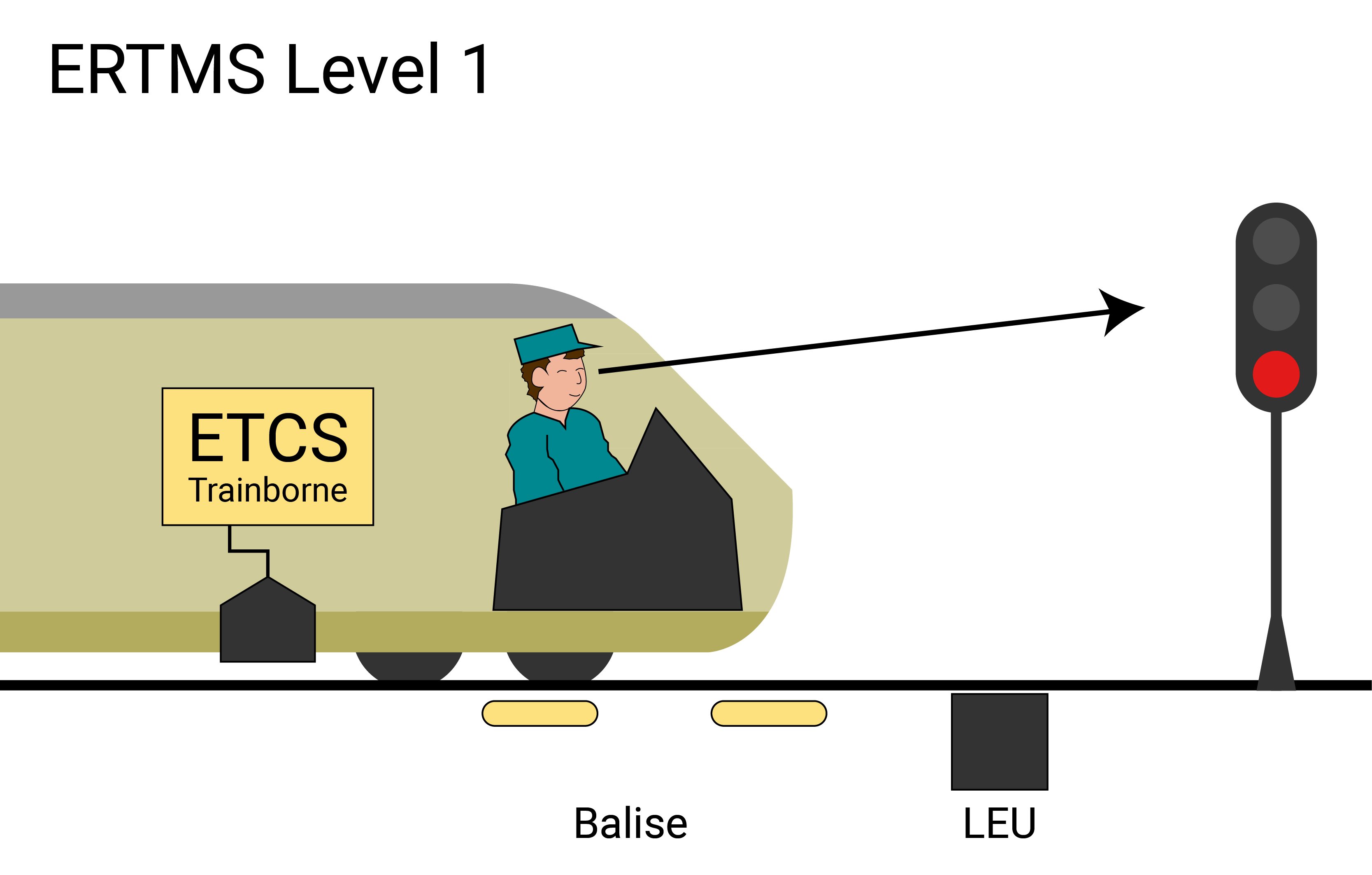 ERTMS (European Railway Traffic Management System) uses train characteristics like weight and braking distance, which are specific per train and can have a wide variety. When implemented ERTMS will also use new ways to communicate via GSM-R, so the train driver can get his information directly from the control centre into his train, eventually signals next to the tracks will not be needed anymore. The current ATP (Automatic Train Protection) is a more conservative system compared to ERTMS. Below we will show you how the system works in the three levels of possible implementation.Level one ERTMS is characterised by the one-way point-to-point communication from the control centre to the traindriver, using the signals next to the tracks. The tracks are divided in fixed blocks and these are either free or occupied by a train, measured via sensors in or next to the tracks, and relayed back to the control centre via a wired network. The Balises between the tracks under the train are transponders to pass on information to the train. This connects to the conventional ATP and control centre via the Lineside Electronics Unit(LEU).
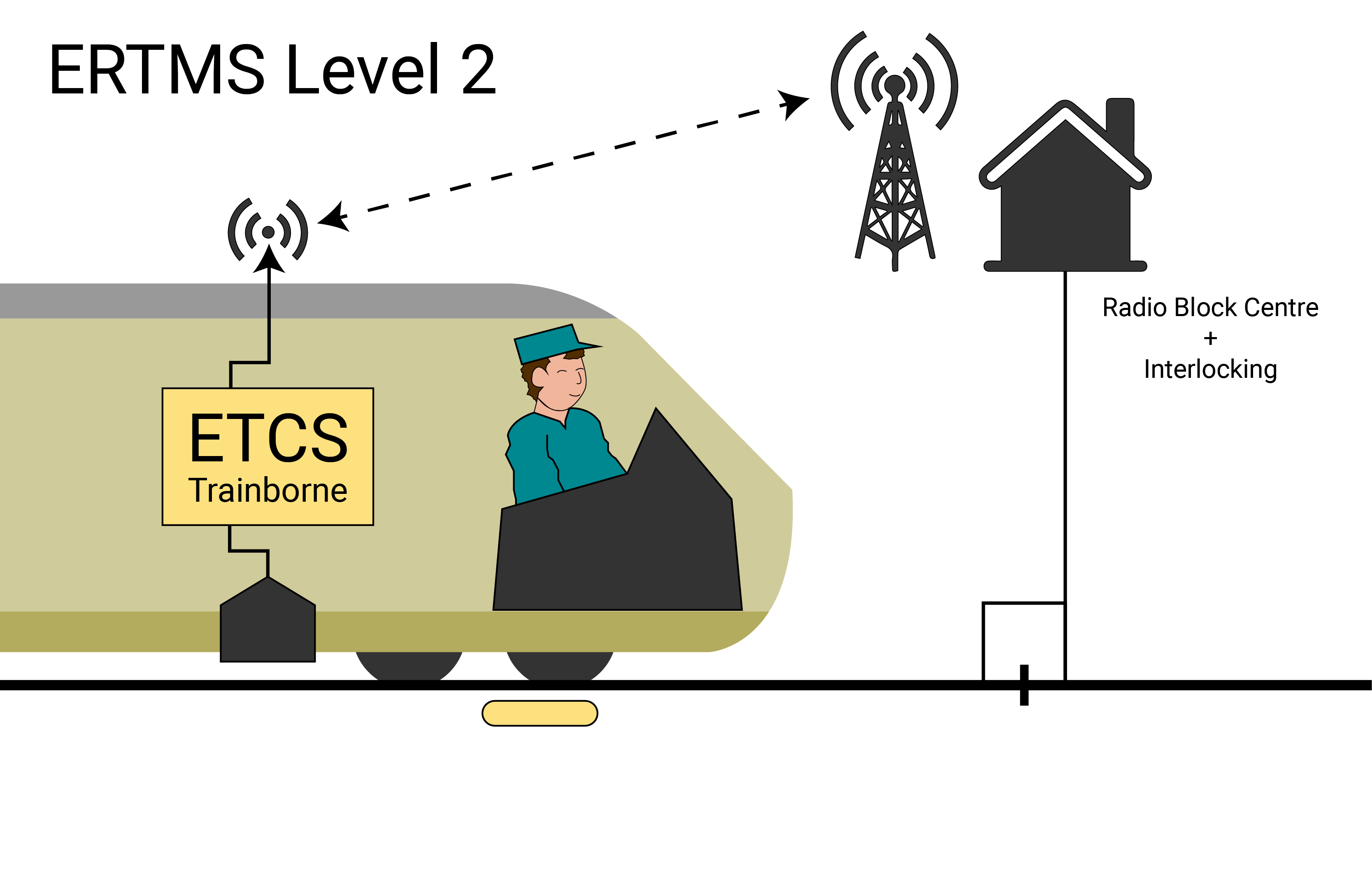
This level has continuous two-way communication with the control centre via GSM-R, a special radio communication service for rail. All the information needed is given via GSM-R and displayed directly in the train. This means that the signals next to the track are no longer needed. The location of the train is still relayed back via the sensors in the tracks, and the system still uses the before mentioned blocks.
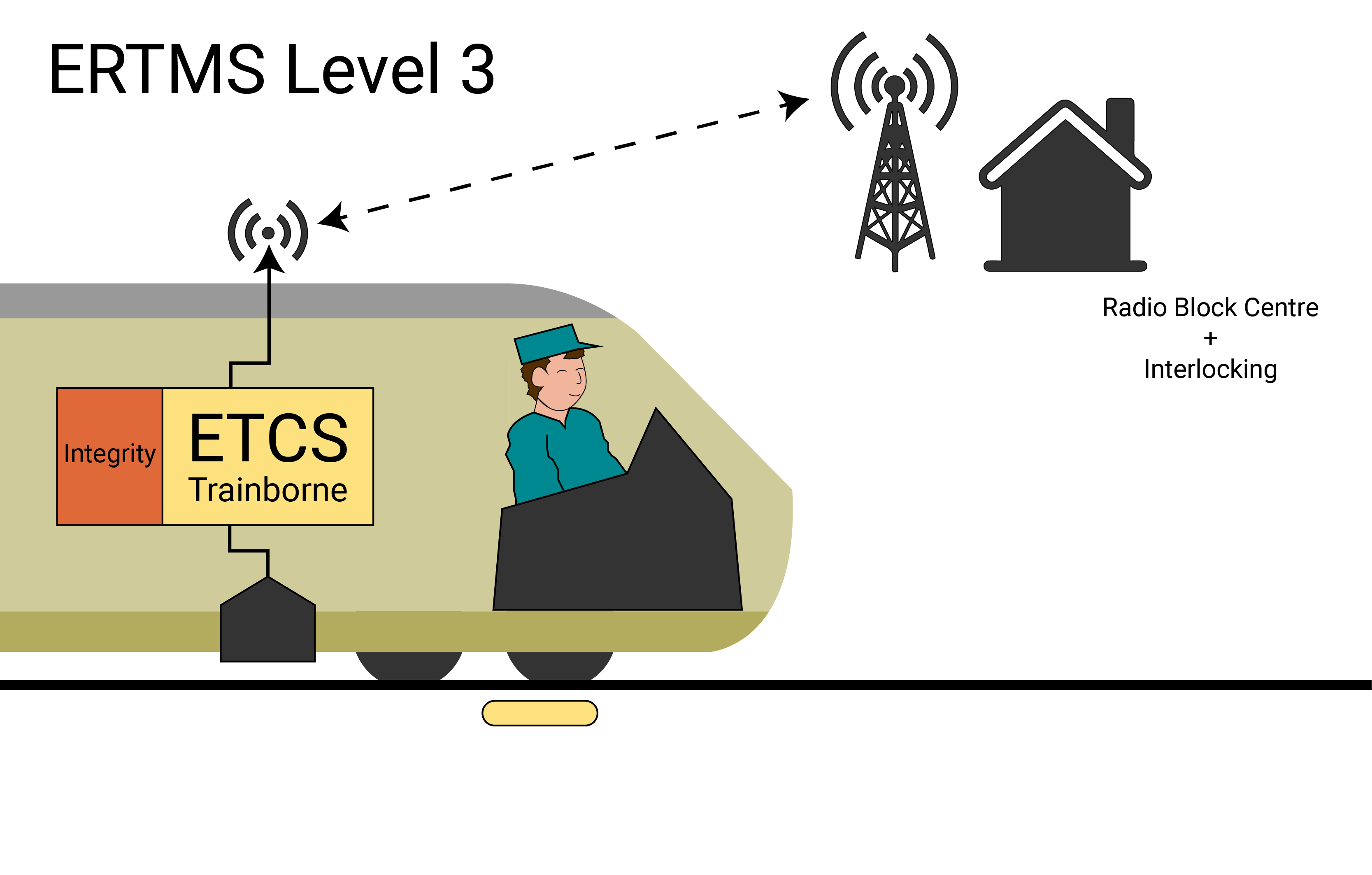 The highest level of ERTMS also uses the GSM-R and directly displays the information in the train. The location of the train is now also relayed back via GSM-R. Additionally the train also checks its own integrity, in case one of its cars breaks loose. This is required because the sensors in the tracks are no longer used. Due to the new location tracking the fixed block system can be adjusted for a moving block system, giving more capacity.
In the advanced ProfEd course on operations we will go further into depth on ERTMS and other safety control systems. If you would like to already share more details on ERTMS and the planned implementation within Europe or other systems used around the world.

Railway Engineering: An Integral Approach by TU Delft OpenCourseWare is licensed under a Creative Commons Attribution-NonCommercial-ShareAlike 4.0 International License.
Based on a work at https://ocw.tudelft.nl/courses/railway-engineering-integral-approach/.