


4.2.2 Traditional Scheduling in Computer Systems
Course subject(s)
4: Resource Management and Scheduling
We have introduced, in Module 4.2.1, the idea that available resources must be managed well, to satisfy both the system users and the resource operators. For the remainder of Module 4, we focus on short-term resource management and scheduling (RM&S), particularly on (short-term) scheduling. Traditional scheduling offers many techniques for designing, analyzing, developing, deploying, and operating scheduling in computer systems. These are the focus of this Module 4 section.
Two major fields of inquiry focus on traditional scheduling: Operations Research (Systems Analysis) and Operating Systems (part of Computer Systems). We address them in turn.
Basic Concepts from Operations Research and Systems Analysis
Scheduling has a long tradition in operations research and systems analysis. Numerous meaningful theoretical results, especially related to understanding how schedulers work and to finding optimal schedulers, have appeared steadily and have impacted computer systems from the 1950s on.
One strong conceptual result from this field relates to the following design principle:
| Design principle: Separate mechanism from policy. |
The mechanism describes what the system does, mechanically, once it encounters the appropriate trigger, such as the periodic clock tick or the sudden arrival of a new workload. A typical scheduling mechanism could be to add incoming workload to the queue, or to retrieve one job from the queue so it can be allocated resources; the queue is an abstract object store that can hold information about jobs (and others), and both operations described in this paragraph are typical of Queueing Theory.
The policy guides how the mechanism will take decisions. In many RM&S frameworks, both theoretical and operational, the policy is encoded as an algorithm, with precisely specified input and output.
Operations Research separates many scheduling problems by type of problem, for which typically only a few mechanisms exist, and then by class of policy, for which typically many policies exist. This allows for efficient exploration of the vast design space of mechanisms and policies.
The separation of mechanism from policy is also highly desirable in practice, as it enables the separation of concerns, clear code, and the ability to switch the policy at runtime with minimal complexity. Consequently, it is much used in computer systems.
Little’s Law: Relating Queue Length, Workload Arrival Rate, and Service Duration
A strong result in Queueing Theory is Little’s Law, a theorem that relates (i) the queue length or how many jobs are waiting on average in the computer system, (ii) the workload arrival rate or how quickly new jobs arrive to the computer system, as a long-term average, and (iii) how long it takes for the system to complete a job, as a long-term average.
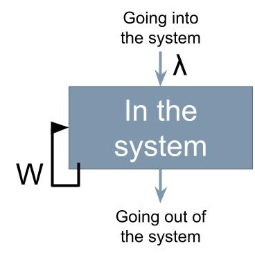
Little’s Law captures this relationship through a formula:
L = λ W,
where L is the expected number of jobs in the queue, lambda (λ) is the arrival rate, and W is the job completion time. The figure depicts the process that relates these variables.
The formula provides a broad analytical tool, which is independent of the statistical properties of the arrival process and of the completion process.
However, the formula only holds under strict assumptions that the system is stable, that jobs cannot be pre-empted (stopped) once they started, and more generally about how heterogeneous the workload, resources, and mechanisms to manage them can be.
The strong assumptions used in operations research and systems analysis, both explicit and implicit, limit their applicability in practice in distributed systems, beyond the most convenient settings.
Basic Concepts from Operating Systems
More closely related to the scheduling work used in distributed systems today, Operating Systems (OS) have been the original fertile ground for scheduling techniques in computer systems. Several essential concepts originated early on (as early as the 1950s) and remain active today:
- Operationalizing (making feasible in practice) the separation of the scheduling mechanism (the what) from the scheduling policy (the how). Basic mechanisms include the (mere) execution of a job, but more sophisticated approaches can include other resource management techniques, such as replication, migration, offloading, partitioning, and other related techniques. Modern scheduling mechanisms in OS can include advanced capabilities to prioritize and order jobs, to get designated jobs completed by a specific deadline, to use accounting for users and groups of users, etc. These mechanisms represent extensions and departures from classic Operations Research. Conversely, there exist hundreds of meaningful scheduling policies, but only a few are much used in OS in practice.
- Agreeing on the basic unit of scheduling. Many operating systems schedule tasks, which can encapsulate work that runs on a processor, typically the CPU. Tasks can be combined into jobs, but this happens outside the job of the operating system’s scheduler, e.g., by chaining together jobs through the Linux pipe operator.
- Agreeing on the basic goals for scheduling. Goals can be functional (see Module 2), such as “schedule a task”, or non-functional (see Module 3), such as “return a decision with a deadline of 1 hour”.
Today, for small computer systems, where a single operating system guides the entire operation – think Linux or MacOS for your laptop -, it is common to employ three basic goals for scheduling:
- (Functional) Schedule the entire workload, e.g., “schedule all tasks”. Schedulers must not let tasks starve for resources indefinitely.
- (Functional) Optimize or satisfice for typical metrics, e.g., turnaround time and utilization, and for typical needs, e.g., prioritizing some jobs over others. Most schedulers make decisions at runtime, so the time needed to reach optimal decisions is prohibitive or even infeasible. This leaves as an alternative for the scheduler the goal of satisficing, that is, of finding a good, feasible trade-off between conflicting metrics and needs.
- (Non-functional) Compute a schedule subject to operational and performance constraints, e.g., in a matter of seconds up to minutes.
Basic Scheduling Policies from Operating Systems
Consider the basic mechanism of scheduling tasks that stream into the system without prior notification, where arriving tasks are added to an unlimited queue and removed according to the policy. Many scheduling policies exist for this mechanism, each taking as input the current state of the queue and returning (selecting) one task to be allocated resources. (For a comprehensive treatment of this mechanism, see Andrea and Remzi Arpaci-Dusseau, Operating Systems: Three Easy Pieces, Chapters 7-10.)
We explore in the following three such policies, aiming to showcase how policies work, why the policy matters, and the interplay between policy and workload.
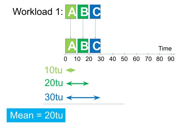
Figure 1. Execution of a simple workload of three uniform tasks, subject to the FCFS policy.
In our exploration, the system consists of one CPU and can run one task at a time. Once a task started, the scheduling mechanism will not interrupt it. The scheduling policy, triggered by the scheduling mechanism each time the queue is not empty and the CPU is free, selects exactly one task from the queue and allocates the CPU for its execution. For simplicity, we assume the time needed for the policy to make a selection, for the selection to be enforced so that the task starts running, and cleanup after the task is complete so the CPU becomes again ready to run the next task, is zero in each case; in other words, the overhead for these activities is negligible.
The First Come, First Served (FCFS) — or First In, First Out (FIFO) — selects tasks from the queue with the earliest arrival time. At each selection point, the oldest task in the queue will be selected. Figure 1 depicts the typical operation of this policy, for a simple workload where three tasks, each requiring 10 time units (TUs) to complete in this computer system once they started to run; we label this workload Workload 1. All tasks arrive at the same time, which for convenience we label as time zero (0). We see a first issue: the three tasks arrived simultaneously, so selecting one can be difficult. So let’s assume that tasks never arrive at exactly the same time, and there is a small difference between their arrivals, so that task A arrives slightly before task B, which arrives slightly before task C. Still, the difference is negligible relatively to the TU, e.g., microsecond vs. millisecond. (This does not lose generality, because we can employ another mechanism (and policy) when tasks can arrive at exactly the same time – which happens very rarely in a small computer system, but, unless timestamping allows for very high resolution, can happen in larger-scale systems. Then, simultaneously arriving tasks can be sorted by their unique identifiers and the selected task has the lowest identifier; here, A, then B, then C.)
The scheduling mechanism first invokes the FCFS policy and selects task A. This task runs on the CPU from the current moment, 0, until it completes its required 10 TUs, so it will finish at 10 TUs. While task A is running, both tasks B and C are waiting in the queue, unable to make progress.
After task A completes, the scheduler invokes the FCFS policy, which selects task B. Task B then runs for its required 10 TUs, so it finishes at 20 TUs.
Last, task C starts running and finishes when the time elapsed reaches 30 TUs.
Overall, starting from the time of 0 TUs, when the tasks arrived in the system, task A took 10 TUs to complete, task B took 20 TUs, and task C took 30 TUs. On average, each task too 20 TUs to complete; this is the average (arithmetic mean) turnaround time. This is about twice the actual runtime of the tasks.
What happens with the average turnaround time if the first arriving task, A, is long, for example, it takes 40 TUs to complete? Take a minute to compute what happens here. We label this workload Workload 2.
For Workload 2: Task A takes 40 TUs, so it completes after 40 TUs. Tasks B and C complete after 50 TUs and 60TUs, respectively. The average runtime for Workload 2 is much higher than for Workload 1, 40 TUs vs. 20 TUs.
In this case, the turnaround time of task A is equal to its runtime, because A does not wait at all in the queue. In contrast, the turnaround time of tasks B and C is much longer than their required runtime, by a factor of 5 and 6, respectively.
Should short tasks be punished this way for arriving just after long tasks? Could a different scheduling policy do better? Enters…
The Shortest Job First (SJF) policy schedules one-task jobs, selecting from the queue the task with the shortest required runtime.
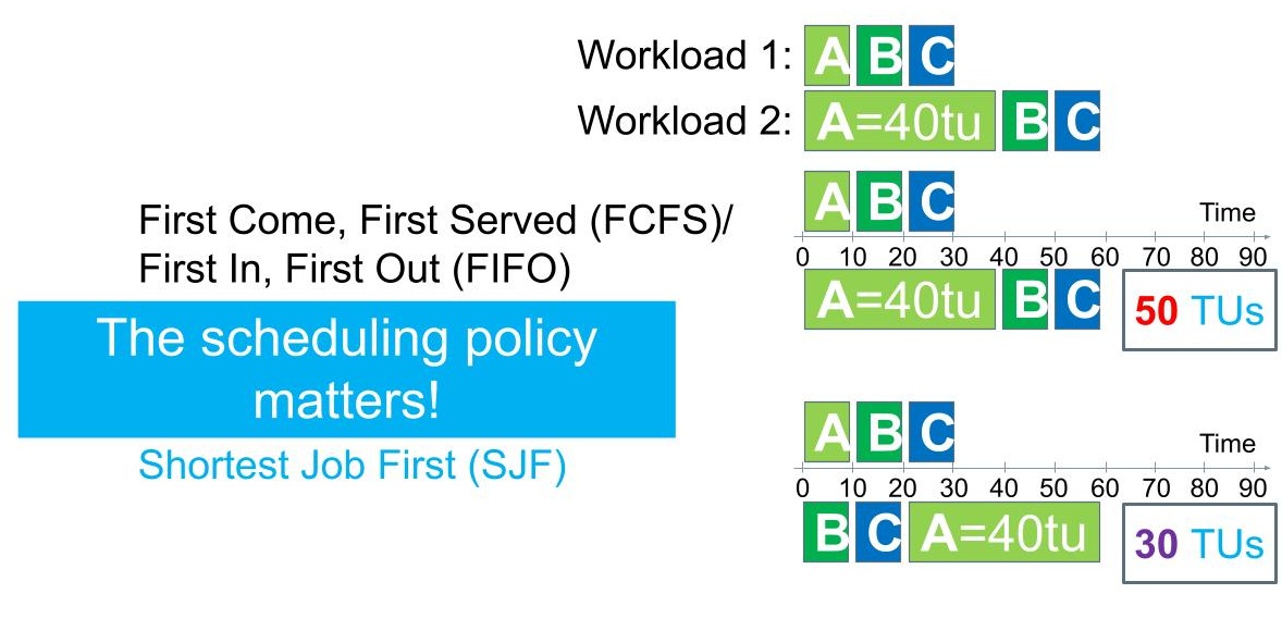
Figure 2. Execution of two simple workloads, exemplifying the performance impact of the scheduling policy.
Consider the example illustrated in Figure 2, which contrasts the execution of the two simple workloads we encountered in this section, subject to the two policies FCFS and SJF. For Workload 1, the policies deliver the same selection, and thus lead to the same performance metrics.
For Workload 2, at least one task, A, is much longer than the others, so SJF can perform its selective function properly. It selects first task B, then task C, and only then task A, which is the reverse order of the selections made by FCFS. SJF significantly improves the average turnaround time, achieving 30 TUs vs. the 50 TUs achieved by FCFS. Strong theoretical results indicate that, under strict assumptions, SJF is nearly optimal, whereas FCFS is generally not.
We conclude from this example the scheduling policy matters.
So far, all the tasks to become the object of selection by scheduling policy were in the queue at the time of the first selection. What happens if we consider a different arrival process?
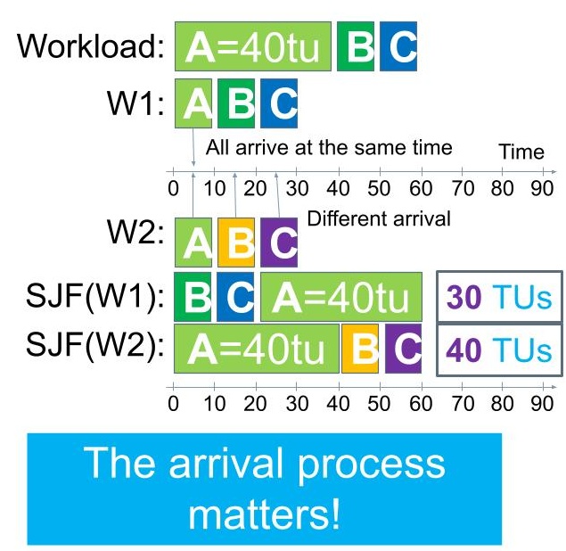
Figure 3. Execution of two simple workloads, exemplifying the performance impact of the arrival process.
Consider the example illustrated in Figure 3, in which a workload arrives comprised of the same tasks (A, of 40 TUs, and B and C, of 10 TUs each), but with different arrival patters. For workload W1, the arrival pattern is that all tasks arrive at the same time. In contrast, for workload W2, we see a different arrival pattern, where task A arrives after zero (0) TUs, task B arrives after 10 TUs, and task C arrives after 20 TUs.
The system uses the same scheduling policy, SJF. For workload W1, the system selects as in the previous example, first task B, then task C, then the much longer task A. The average turnaround time is 30 TUs.
For workload W2, the SJF policy selects task A from a queue that includes only. Although we can see this task is much longer than the other two, the SJF policy can only select from the tasks that it sees, and thus is forced to select task A as the shortest in the current queue. Once task A has been selected, it is immediately allocated the CPU, where it runs until completion. Only then does the scheduling mechanism invoke the SJF policy again, selecting task B from a queue with tasks B and C in it, and finally selecting task C. The average turnaround time for W2 is 40 TUs (note, e.g., task B arrives after 10 TUs and completes after 50 TUs); this is significantly higher than what we observed for W1.
We conclude from this example the arrival process matters.
More Advanced Concepts from OS
Many advanced scheduling concepts stem from the OS community, which apply today in distributed systems.
In the section about Basic Scheduling Concepts from OS, we saw that often our exemplary jobs aligned with a time unit increment of 10 TUs. Many modern OSs consider a time slice, a time unit of time until OS interrupts (preempts) running tasks, allowing multiple tasks to share the much fewer processing cores. Time slices are used by many common schedulers, e.g., in Linux. For example, the Round Robin scheduling policy, used in the earliest versions of Linux, alternates which task receives CPU access during the next time slice.
The modern OS differentiates strictly between interactive and batch tasks, and possibly other scheduling classes. For example, in Linux, the scheduling system offers mechanisms and allows setting policies for interactive (real-time) tasks, batch (non-real-time), and in-between non-preemptible tasks.
Priorities can be assigned to different tasks (and scheduling classes, to begin with), which can be used by the scheduling mechanism and/or the scheduling policy to determine which task should get priority to using the available resources.
As a more general concept than priorities, proportional share and fair-share scheduling aim to give tasks access to resources proportional to what they should receive. For example, the Linux Completely Fair Scheduler (CFS) scheduler considers for each task (or group) the virtual runtime the task has already consumed from the system. At each decision, CFS selects the task with the least amount of virtual runtime; the implementation of this operation is based on the red-black-tree data structure, which offers good performance. Running tasks are pre-empted by the system or yield their remaining time in the current time slice.
These concepts are not only advanced on their own, but they also need to be combined to produce useful results. For example, the CFS also supports jobs comprised of multiple and even many tasks, thus enabling group scheduling. Groups of tasks share their virtual runtime, preventing a task can spawn many small tasks, each of which will have a very low virtual runtime and thus execute before other tasks in the system. Furthermore, CFS uses priorities to decay (reduce by a factor) the virtual runtime for each task, decreasing the record of consumed resources more for jobs with better priority.
Many more concepts exist, including a notion of scheduling tasks across multiple processing cores. However, as we will see, distributed systems require much more than scheduling across multiple processing cores.

Modern Distributed Systems by TU Delft OpenCourseWare is licensed under a Creative Commons Attribution-NonCommercial-ShareAlike 4.0 International License.
Based on a work at https://online-learning.tudelft.nl/courses/modern-distributed-systems/