Non-linear least squares estimation 

Let the non-linear system of observation equations be given by:

\[E \{ \begin{bmatrix} \underline{y}_1\\ \underline{y}_2\\ \vdots\\ \underline{y}_m \end{bmatrix}  \} = A(x) = \begin{bmatrix} a_{1}(x)\\ a_{2}(x)\\ \vdots\\  a_{m}(x) \end{bmatrix}\]

This system cannot be directly solved using the weighted least squares or the best linear unbiased estimators. Here, we will introduce the non-linear least squares principle, based on a linearization of the system of equations. For the linearization we need the first-order Taylor polynomial, which gives the linear approximation of for instance the first observation \(y_1 = a_1(x)\) at \(x_{[0]}\) as:

\[y_1\approx a_1( x_{[0]})+ \partial_{x_1} a_1(x_{[0]})\Delta x_{[0]}+ \partial_{x_2} a_1(x_{[0]})\Delta x_{[0]}+ \ldots + \partial_{x_n} a_1(x_{[0]})\Delta x_{[0]}\]

where \(\Delta x_{[0]} = x- x_{[0]}\) and \(x_{[0]}\) is the initial guess of \(x\).

The difference between the actual observation \(y_1\) and the solution of the forward model at \(x_{[0]}\) is thus given by:

\[\begin{align} \Delta y_{1[0]} &= y_1- a_1(x_{[0]}) \\ &\approx \left[ \partial_{x_1} a_1(x_{[0]}) \quad \partial_{x_2} a_1(x_{[0]}) \quad \ldots \quad \partial_{x_n} a_1(x_{[0]})\right]\Delta x_{[0]} \end{align}\]

We can now obtain the linearised functional model:

\[\begin{align} E\{\begin{bmatrix} \Delta \underline{y}_1 \\ \Delta\underline{y}_2 \\ \vdots \\ \Delta\underline{y}_m \end{bmatrix}_{[0]}\} &=\begin{bmatrix} \partial_{x_1} a_1(x_{[0]}) &\partial_{x_2} a_1(x_{[0]}) & \ldots & \partial_{x_n} a_1(x_{[0]}) \\ \partial_{x_1} a_2(x_{[0]}) &\partial_{x_2} a_2(x_{[0]}) & \ldots & \partial_{x_n} a_2(x_{[0]}) \\ \vdots & \vdots  & \ddots  & \vdots\\ \partial_{x_1} a_m(x_{[0]}) &\partial_{x_2} a_m(x_{[0]}) & \ldots& \partial_{x_n} a_m(x_{[0]}) \end{bmatrix}\Delta x_{[0]} \\ &= J_{[0]}\Delta x_{[0]}\end{align}\]

with Jacobian matrix \(J_{[0]}\).

And this allows to apply best linear unbiased estimation (BLUE) to get an estimate for \(\Delta x_{[0]}\):

\[\Delta \hat{x}_{[0]}=\left(J_{[0]}^T Q_{yy}^{-1} J_{[0]} \right)^{-1}J_{[0]}^T Q_{yy}^{-1}\Delta y_{[0]}\]

since the Jacobian \( J_{[0]}\) takes the role of the design matrix \(A\) and the observation vector is replaced by its delta-version as compared to the BLUE of the linear model \(E\{\underline{y}\} = Ax\).

Since we have \(\Delta x_{[0]} = x- x_{[0]}\), an “estimate” of \(x\) can thus be obtained as:

\[x_{[1]}=x_{[0]}+\Delta \hat{x}_{[0]}\]

However, the quality of the linear approximation depends very much on the closeness of \(x_{[0]}\) to \(x\). Therefore, instead of using \(x_{[1]}\) as the estimate, we repeat the process with \(x_{[1]}\) as our new guess. This procedure is continued until the \(\Delta \hat{x}_{[i]}\) becomes small enough. This is called the Gauss-Newton iteration procedure, and is shown in the scheme below.

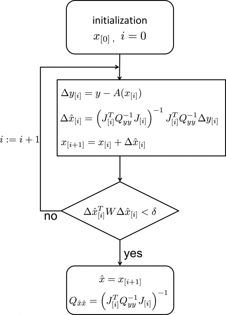
In this scheme you can see that as stop criterion

\[\Delta \hat{x}_{[i]}^T W \Delta \hat{x}_{[i]} < \delta\]

is used. The weight matrix \(W\) can be set equal to for instance the identity matrix, but a more logical choice may be the inverse normal matrix \(N_{[i]}=J_{[i]}^T Q_{yy}^{-1} J_{[i]}\). The threshold \(\delta\) must be set to a very small value. 

Once the stop criterion is met, we say that the solution converged, and the last solution \( x_{[i+1]}\) is then finally used as our estimate of \(x\). 

Remarks and properties

There is no default recipe for making the initial guess \(x_{[0]}\); it must be made based on insight into the problem at hand. A good initial guess is important for two reasons:

• - a bad initial guess may result in the solution NOT to converge;
• - a good initial guess will speed up the convergence, i.e. requiring fewer iterations.

In the iteration scheme the covariance matrix of \(\hat{x}\) was given by:

\[Q_{\hat{x}\hat{x}}=\left(J_{[i]}^T Q_{yy}^{-1} J_{[i]} \right)^{-1}\]

In fact, this is not strictly true. The estimator \(\underline{\hat x}\) is namely NOT a best linear unbiased estimator of \(x\) since we used a linear approximation. And since the estimator is not a linear estimator, it is not normally distributed. 

However, in practice the linear (first-order Taylor) approximation often works so well that the performance is very close to that of BLUE and we may assume the normal distribution.