


4.6 Mathematical formulas in LaTeX
Course subject(s)
4. Reporting your findings
On this page we will introduce you to the most common building blocks of mathematics in LATEX. You will practice with this in the exercises. In the next page, we will discuss how you can include these formulas in your report.
Powers, exponents, superscripts and subscripts
Mathematics contain often powers of numbers, exponentials, superscripts and subscripts. Examples of these are et, x2 and X1.
In LATEX, you can obtain this by using the ^ and the _ symbol. The three examples above are generated as follows:
- e^t results in et.
- x^2 results in x2.
- X_1 results in X1.
It might happen you want more than one symbol or letter to display as a superscript or subscript. In this case you need to group all symbols together using curly braces, like in the next examples:
- e^{-0.7t} results in e−0.7t.
- X_{1,\text{eq}} results in X1,eq.
Note that letters are displayed slanted by LATEX by default in mathematics. If you want to include non-slanted letters, such as eq in the example, you can use the command \text{…}.
Different uses of formulas
The code for the mathematics above is not directly usable: in LATEX mathematical formulas must be written in math mode. LATEX recognises you want math mode by using some special commands before and after the formula.
Within a scientific report, you can think of several places and ways to display mathematics. Three of these are:
- In the text as part of a sentence;
- As an unnumbered equation;
- As a numbered equation.
We will discuss each of this in the following.
Inline formulas
Mathematics in the text as part of a sentence is called inline math in LATEX. To add such mathematics, you must put your mathematical code between special symbols. There are two options for this:
- Put the code between $ and $;
- Put the code between \( and \).
You can choose which ever one you like. As an example, the code
An example of an inline formula is $\frac{dP}{dt} = 0.7 P(t)$.
is compiled as
![]()
by LATEX. As you can see, the fraction is displayed relatively small. If you want bigger symbols, you can add \displaystyle after the opening symbol of the inline math. This results in
![]()
Unnumbered equations
If you want to draw more attention to a certain formula, you can give the formula its own line, like this:
![]()
To achieve this in LATEX, again, three options exist:
- Put the code between \[ and \];
- Put the code between $$ and $$;
- Put the code between \begin{equation*} and \end{equation*};
Unnumbered equations are automatically in display style, so if you want smaller fractions, you can use the command \tfrac instead of \frac or \dfrac(see also below).
(see also below).
Numbered equations
If you want to draw more attention to a certain formula, and also want to refer back to it (it is that important), you should put a number behind the equation. LATEX will do this automatically if you use the following option:
- Put the code between \begin{equation}\label{mytag} and \end{equation}.
If it is the second numbered equation in Chapter 3, this results in:
![]()
If you want to refer back to this equation in your text, use the command \ref in your text. So \ref{mytag} gives you 3.2 in the text. If you want to have parentheses around the number, you can use \eqref instead.
Numbered equations are, just like unnumbered equations in display style.
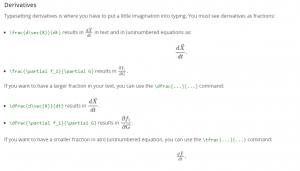
Fractions, roots and vectors
LATEX can also typeset fractions, roots and vectors:
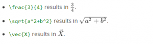
As you can see, you can combine all commands to produce intricate and complex formulas.

Mathematical Modeling Basics by TU Delft OpenCourseWare is licensed under a Creative Commons Attribution-NonCommercial-ShareAlike 4.0 International License.
Based on a work at https://online-learning.tudelft.nl/courses/mathematical-modeling-basics/.