


5.4.1 to 5.4.3
Course subject(s)
5. Monitoring and Maintenance
Decision Making

5.4.1 Dealing with the Data
No matter what kind of monitoring is used, deciding how to deal with the obtained data will be a challenge. Based on the data, a decision needs to be made about the quality of the structure or object. This means information is needed beforehand about how the measured signal (or signals) are related to the quality of the structure. Even though part of this can be modelled, in general, you will always need some real-life data to verify the models before they can be used.
Supervised and unsupervised learning
In the most ideal case, you will collect data of both the undamaged structure and the damaged structure. This is called supervised learning. However, collecting data from a damaged structure can become very costly for a large structure, such as a bridge. You do not want to intentionally damage the whole structure just to get more knowledge about the behaviour. In those cases, only data from an undamaged state of the structure can be used, which is the so-called unsupervised learning.
There are some essential differences in how supervised learning and unsupervised learning can be used. Unsupervised learning is often limited to defining whether damage is present in the system or not. It will not be able to tell the exact location of the damage, the type of damage, the extend of the damage or the expected remaining lifespan of the structure. But with a good supervised learning model, all these questions can be answered.
5.4.2 Dimensionality
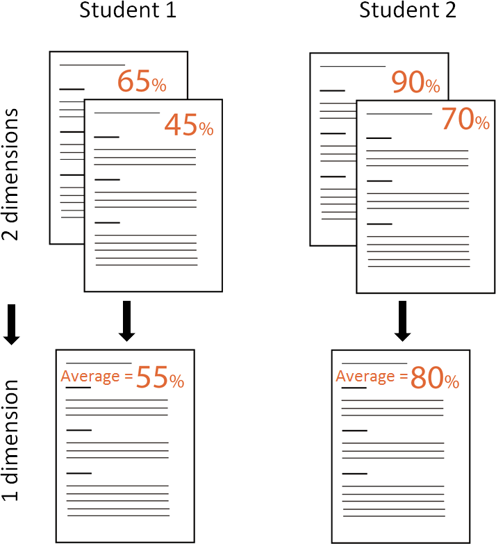
Ideally there will be a single outcome (or so called indicator) from the data processing of a measurement system so it is easy to determine the performance. This is called a one-dimensional indicator. A good example of this is the grade students get on a test. This can simply be evaluated on a single scaling to see whether or not a student passed the test, but also be compared with the results of the other students. Now when we add a second indicator, things start to become more complex. In our student example, this can be a second test for the same course. Now we need to look at both tests to see whether or not a student passed the course and determining the best student becomes a lot harder as well. Ideally, these two indicators are combined back to a single one, to make it easier to do the comparison. An easy solution in this example would be to take the average grading of the two tests as the single indicator, thus reducing the dimensionality back to one.
However, things can become far more complex. In many cases, results from a measurement are nowhere near one-dimensional. When looking at a frequency spectrum for example, we are often talking about more than 100 dimensions. Reducing this to one dimension will diminish all the data into a value, which no longer has any usability. It can even become more extreme when considering black and white images. A black and white image is, in essence, no more than a certain grey-value for each pixel in the image. This means the image has the same number of dimensions as it has pixels, often being millions! Interestingly, computers find it significantly harder to classify a dataset when the dimensionality increases. Humans can still outperform computers on this!
Since in the present day a high number of datasets have to be classified, there is only one solution: reducing the dimensionality of the dataset. This can be done by looking for relations between different data points (or dimensions) of the dataset. When taking an image for example it is clear that not all pixels are randomly determined, but often many pixels are closely related to their neighbour, due to representing the same color. Multiple techniques are available to reduce the dimensionality while maintaining the largest amount of significance of the dataset as a whole. One which is often used is the so called Principle Component Analysis or PCA.
5.4.3 Dealing with Variability
Once the data is reduced to a usable number of dimensions, there is another problem to consider when classifying the data, namely, variability. In our student example from before, even if two students studied equally hard and know exactly the same amount about a subject, they do not necessarily score exactly the same. Many variables could slightly influence the result. For example, how well they slept will influence their performance. This variability also means that the same student taking the test in two different moments will score differently each time.
Something similar is seen in the output of a measurement system. The output on a dimension for a certain state will not always be the same number, but has an uncertainty, often representing a ‘normal distribution’. That’s why we can represent it as an average value and a standard deviation.
Example:
Now let’s consider a one dimensional system, in which we know two states: broken or unbroken.
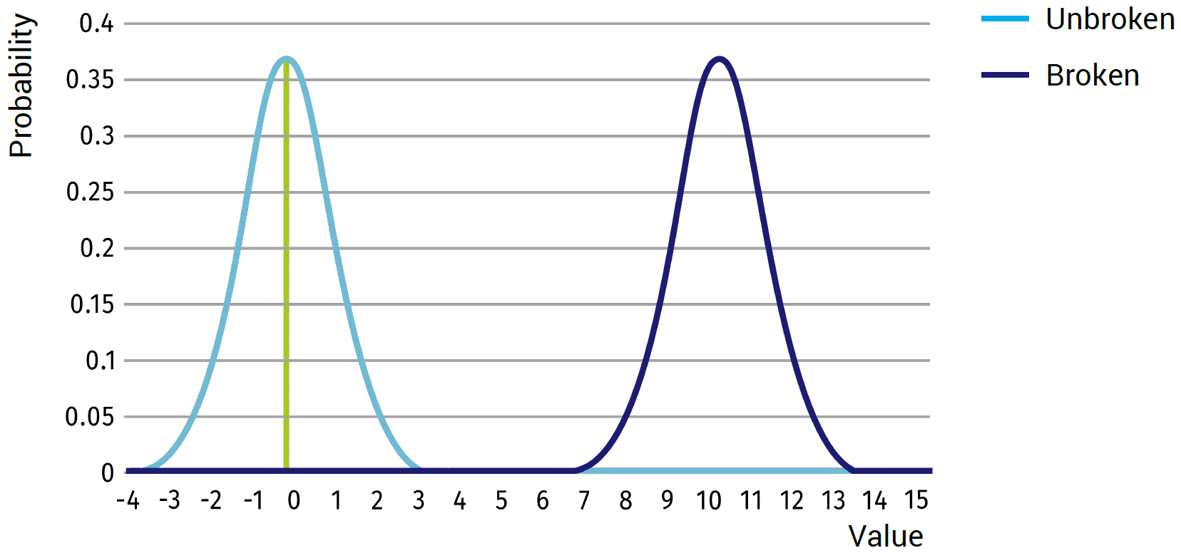
If, for example, the unbroken state will give an average value of 0 with a standard deviation of 1, and the broken state will give an average of 10 with a standard deviation of 1 (see figure above), we can expect that any value around 0 will represent the unbroken state and any value close to 10 will represent the broken state. There will be almost no outcomes in the middle of the two states; thus one would simply tell a computer that anything above 5 is considered broken and below 5 is considered unbroken.
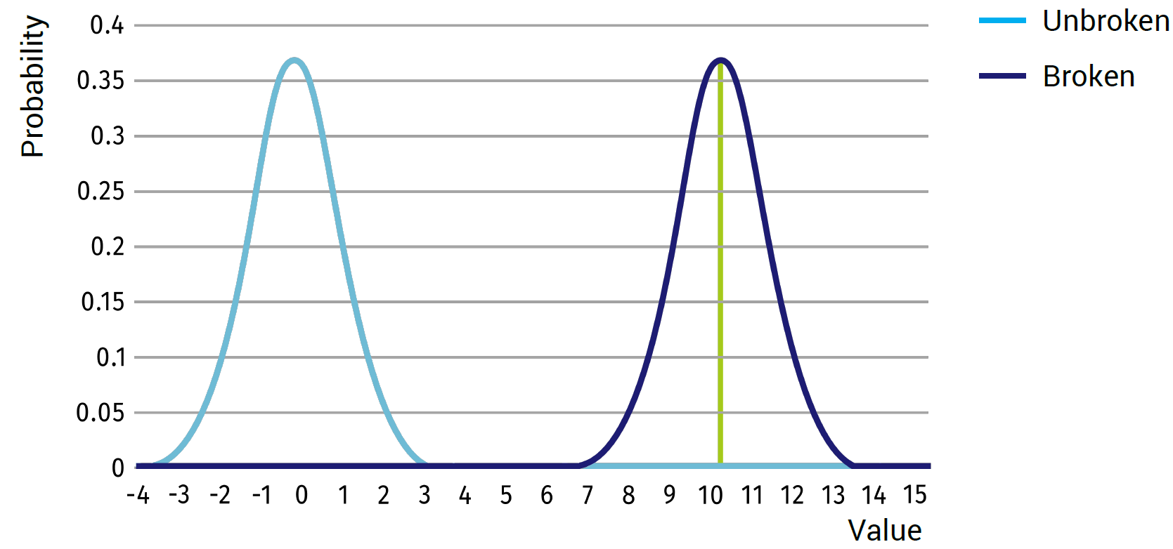
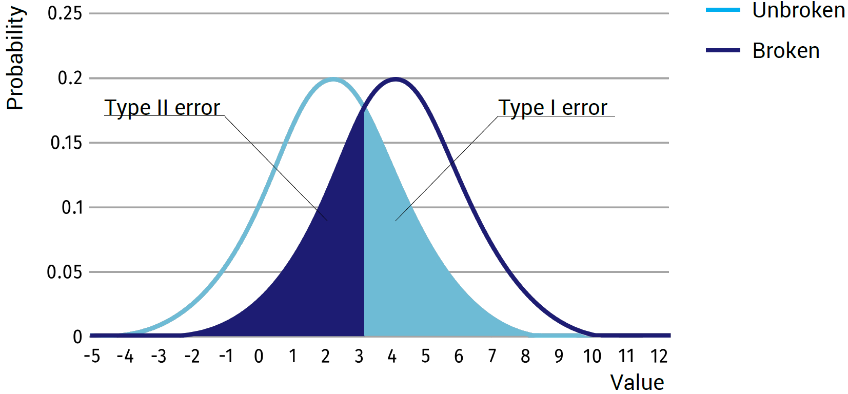
 However, if we now consider the same example, but with an average of 2 and a standard deviation of 2 for the unbroken state and an average of 4 and a standard deviation of 2 for the broken state (see image below), you can see that the results will not always be distinctive in a single case. A value of 3 is likely to occur and could equally be caused by the broken or the unbroken state.
Even the value of 2, though being the average for the unbroken state, might still be caused by the broken state. Therefore, it is not possible to have a single decision boundary to perfectly discriminate between the broken and unbroken cases. Sadly, most cases you will see in real-life will be closer to our second example, thus always resulting in a difficulty to determine a good boundary. Depending on where the boundary is set, a certain amount of false positives (detected as broken, while unbroken in reality), and false negatives (detected as unbroken while being broken) will be in the results.
There are multiple strategies that can be used to determine an optimum decision boundary for the data, such as:
- optimizing the total errors,
- minimizing false positives,
- minimizing false negatives and
- minimizing the total costs of errors.
Which one to use depends on the subject on which the measurement system is being implemented.
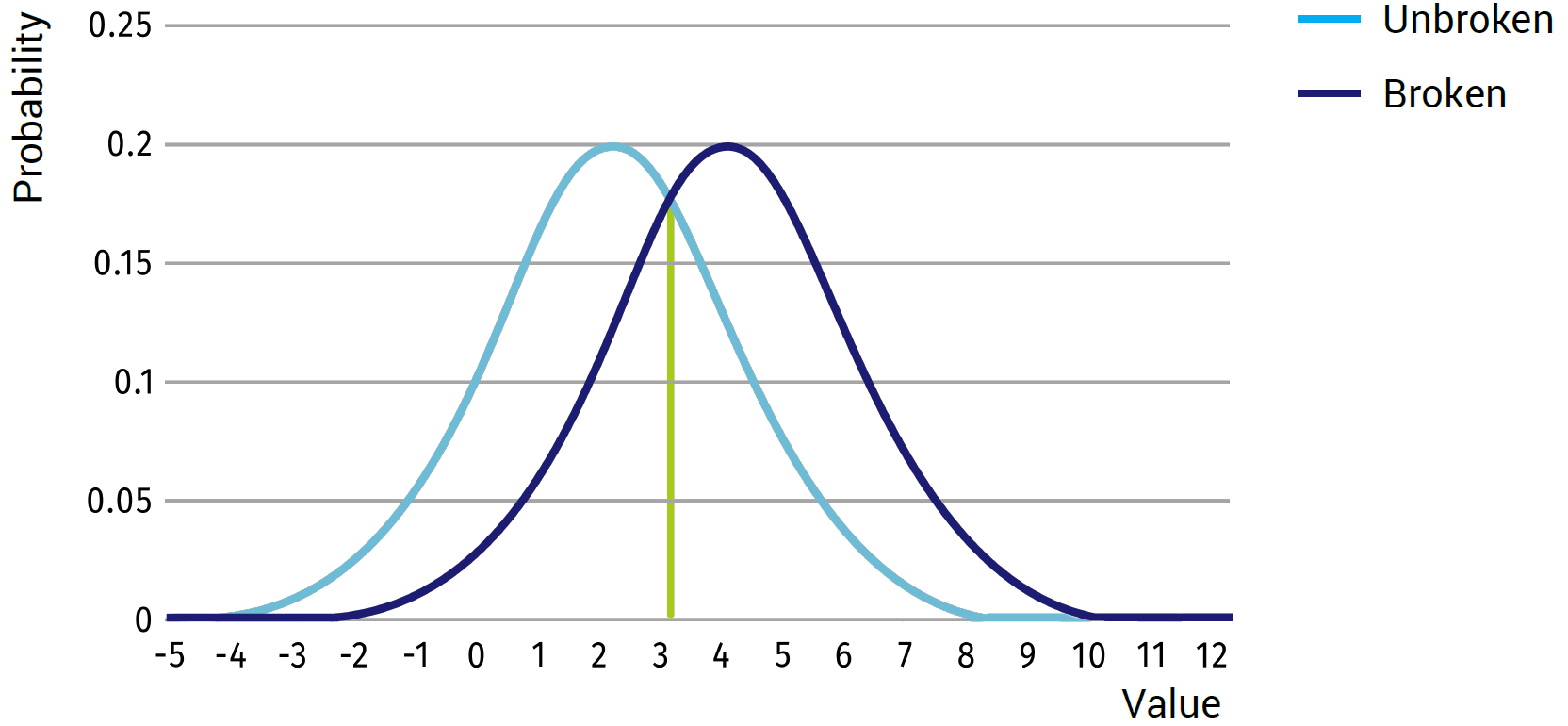
 In cases where the accuracy of the results is of highest importance, one would minimize the total amount of error. To do this, one would simply try to find the intersection between the two probability curves and set the decision boundary at this point (see image below).
In cases where people’s safety plays an important role, such as the airline industry, false negatives are ideally minimized. An airline cannot afford to NOT find a broken part on inspection, which can lead to a crash. Although, due to the character of the normal distribution, in theory, it is never possible to set the chance of a false negative to absolute 0, often the allowable false negative value is set to for example 0.1% thus detecting 99.9% of all broken cases. This, however, inadvertently means that the number of false positives will be considerably higher than necessary, and also the total amount of detection errors is higher than when optimizing the total number of errors.
Minimising False Positives:
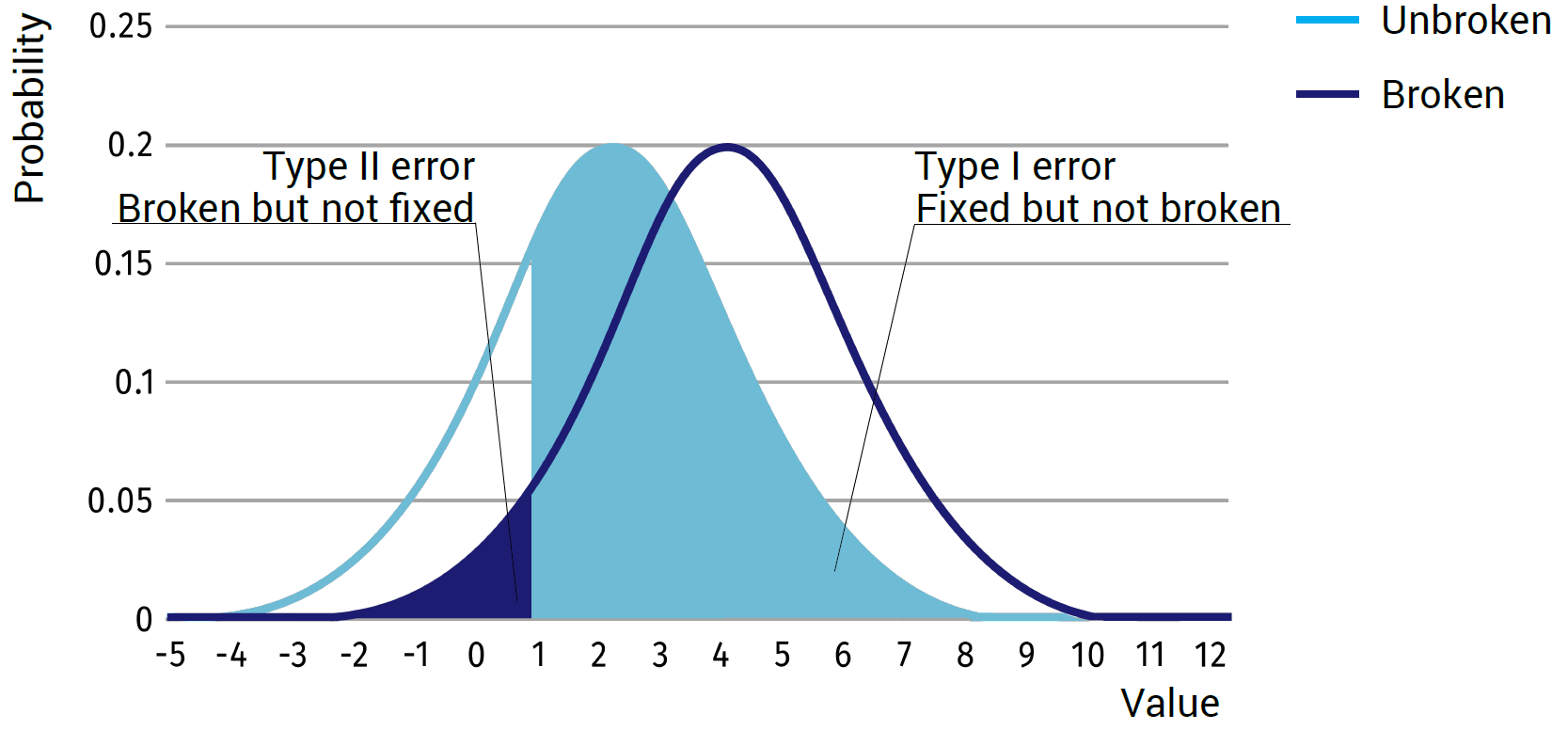
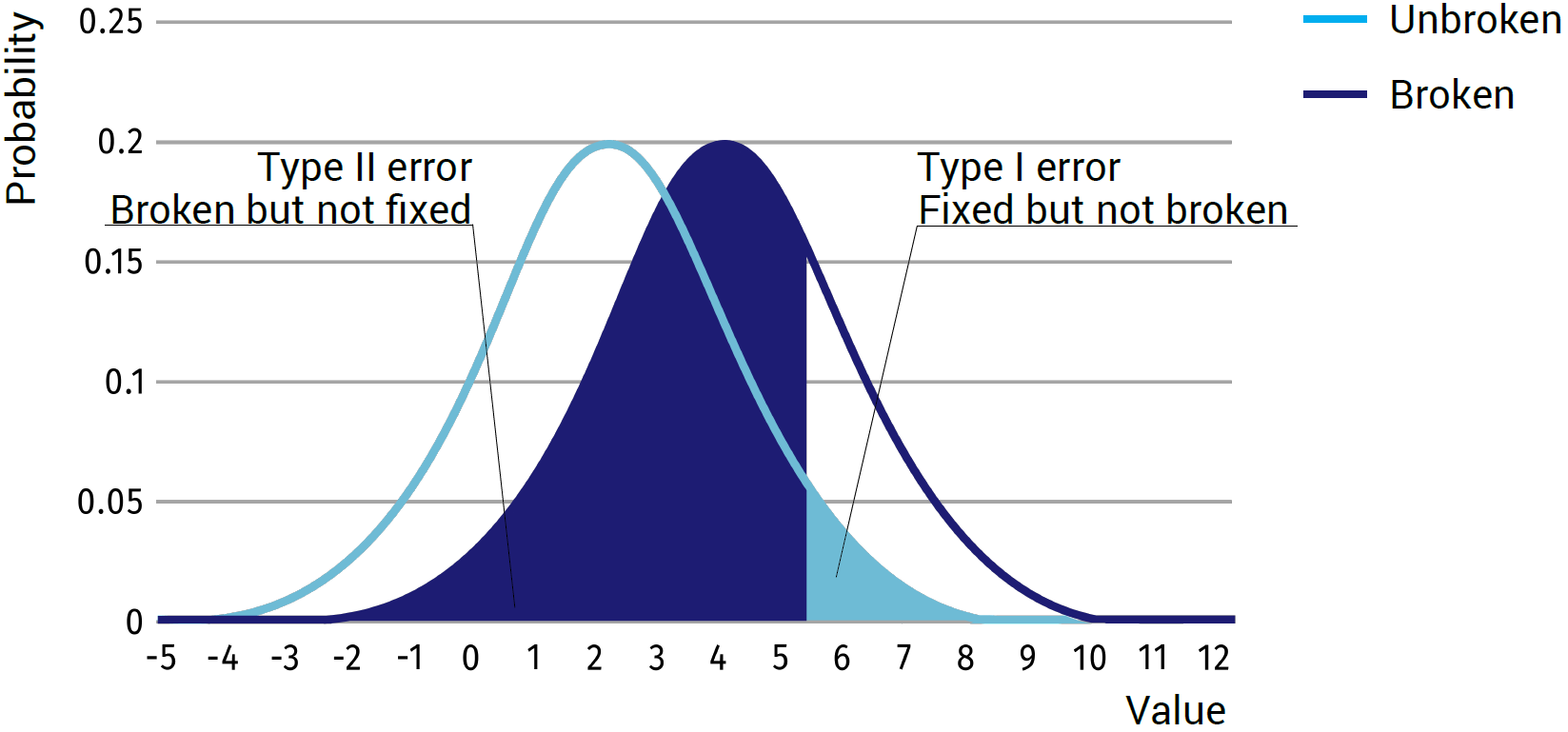
In cases where economic decisions play an important role in the measurement, and failures in the system don’t have considerably large consequences, it is often beneficial to minimize the false positives. By minimizing the number of false positives, the number of repairs that needs to be done is reduced, thus minimizing the maintenance costs. Again it is impossible to set the amount of false positives to absolute 0, thus the allowable false positive value is set to for example 0.1%. Just like in the previous case, this does mean that the number of false negatives is considerably higher than necessary and also the total number of errors is higher than when optimizing on the total amount of errors.
Minimising False Negatives:
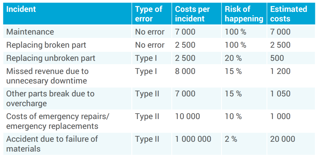
In the last approach, the amount of errors are not optimized (to have them as low as possible), but the total costs are. To do so, the costs for all decisions will need to be determined for the system. The most important two are the costs for the false negative and the false positives. With these costs known, finding an optimum decision boundary for minimizing the costs for the system as a whole is very simple. However, determining the exact costs for these cases is the biggest challenge.

Railway Engineering: An Integral Approach by TU Delft OpenCourseWare is licensed under a Creative Commons Attribution-NonCommercial-ShareAlike 4.0 International License.
Based on a work at https://ocw.tudelft.nl/courses/railway-engineering-integral-approach/.