


6.1 Summary
Course subject(s)
6. Does the estimate make sense?
Precision, as described by the covariance matrix of the estimators, is an important measure of the quality of the estimated parameters. The precision of that is given by:
\[Q_{\hat{x}\hat{x}} = (A^T Q_{yy}^{-1}A)^{-1}\]
- - one or more outliers in the observations \(y\);
- - a systematic bias in (a subset of) the observations \(y\);
- - a wrong assumption regarding the \(A\)-matrix;
- - a wrong assumption regarding the \(Q_{yy}\)-matrix.
All these errors will affect the estimates, and will generally result in larger residuals than in the ‘unbiased’ case (i.e., when none of the aforementioned types of errors is present, and only random errors cause deviations from the truth).
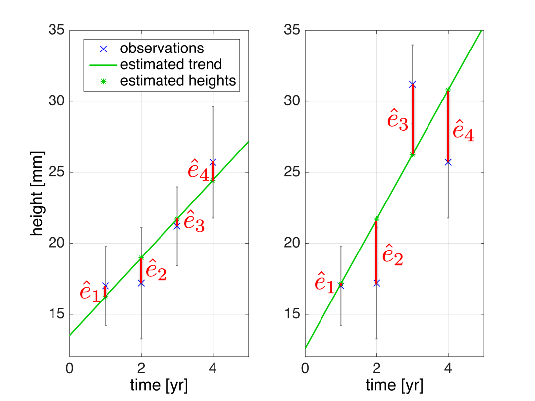
It is important to note that a bias in specific observations may also result in larger residuals for the other observations. Take the example where we fit a line through a number of observations as shown in the figure; if one of the observations contains a large error the effect is that the fitted line is ‘pulled’ towards that erroneous observation (right-hand figure, third observation is an outlier) as compared to the case where the error is absent (left-hand figure); as a consequence especially the residuals of the neighbouring observations may be severely affected.
The so-called overall model test can be used to detect whether an error is present. Its test statistic is given by:
\[ \underline{T} = \underline{\hat{e}}^T Q_{yy}^{-1} \underline{\hat{e}}\]
Intuitively it makes sense to use this as a test statistic since:
- -it compares the size of residuals \(\hat{e}\) (i.e., the estimated random errors) versus the measurement precision \(Q_{yy}=Q_{ee}\);
- - the test statistic is what is minimized to get the estimator providing the ‘best fit’;
- - all residuals are considered.
One or more errors (not being a random error) is/are suspected to be present if the test statistic takes a 'too large' value. The decision when the test statistic is considered too large is made in a probabilistic way. It is known that the distribution of \(\underline{T}\) is the central \(\chi^2\)-distribution (chi-square) with \(m-n\) degrees of freedom:
\[\underline{T}\sim \chi^2(m-n,0)\]
Recall that \(m-n\) is the redundancy, and we see that the distribution of \(\underline{T}\) is only a function of the redundancy.
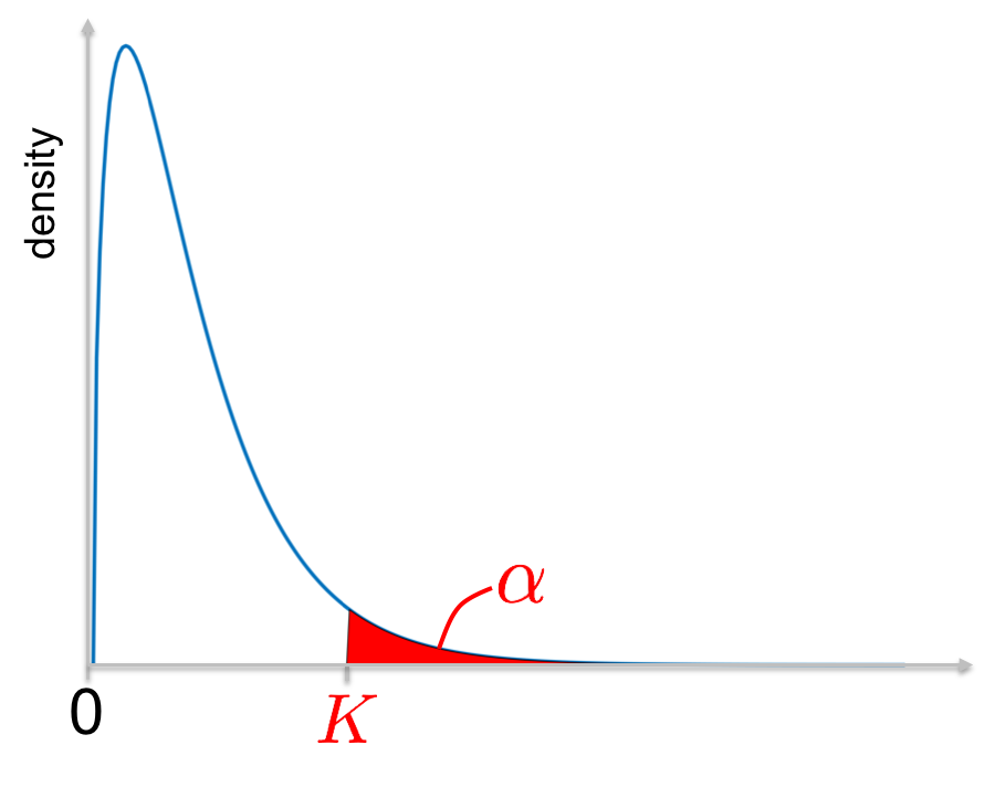
Knowing the distribution, it is possible to evaluate the probability that \(\underline{T}\) is larger than a certain value. The idea is then to choose a small probability, called \(\alpha\) and to find the corresponding value \(K\) such that (see figure):
\[P(\underline{T}>K) = \alpha\]
This implies that it is unlikely that a
The complete procedure is as follows:
- 1. Set up the model: \(E\{\underline{y}\}=Ax;\;\;D\{\underline{y}\}=Q_{yy}\)
- 2. Collect the observations \(y\).
- 3. Estimate the parameters and their precision: \(\hat{x} = (A^T Q_{yy}^{-1} A)^{-1} A^T Q_{yy}^{-1} y\); \(Q_{\hat{x}\hat{x}}=(A^T Q_{yy}^{-1} A)^{-1}\).
- 4. Compute the residuals: \(\hat{e} = y-A\hat{x}\).
- 5. Compute the overall model test statistic: \(T=\hat{e}^T Q_{yy}^{-1}\hat{e}\).
- 6. Check whether \(T>K\).

Observation Theory: Estimating the Unknown by TU Delft OpenCourseWare is licensed under a Creative Commons Attribution-NonCommercial-ShareAlike 4.0 International License.
Based on a work at https://ocw.tudelft.nl/courses/observation-theory-estimating-unknown.