


Food for thought: LSE
Course subject(s)
3. Least Squares Estimation (LSE)
In case we are interested in the linear trend of sea level rise, we have found that the observation equation for an individual tide gauge observation \(y_i\) would be:
\( y_i = l_0 + r\cdot \Delta t_i \)
with \(\Delta t_i\) the time differences with respect to \(t_0\), and the unknown initial sea level \(l_0\) at \(t_0\) and the unknown rate of change \(r\).
The figure shows the record of sea level observations (light blue) based on tide gauge observations, together with 3 'fitted' lines to model the sea level rise as a linear trend.
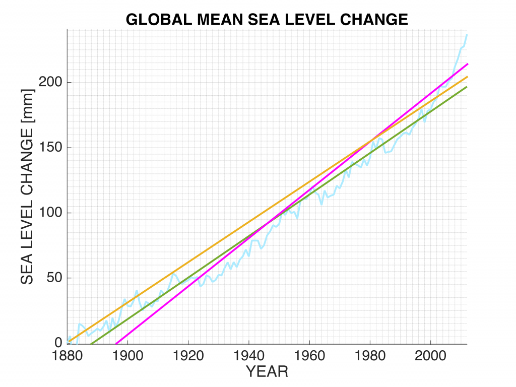
None of these lines fits perfectly to the data, this is due to measurement errors and model imperfections (the sea level variations cannot be simply modeled by a linear trend only). How to deal with this, is the topic of the upcoming parts in this course.
Food for Thought questions to you:
- - Which line ‘fits’ best to the data?
- - What criterion would you use to answer the previous question?
- - How to compute the parameters \(l_0\) and \(r\) for the ‘best fitting’ model?
In this module you will learn how the least squares principle can be used to answer these questions; we'll address them again at the end of this module.

Observation Theory: Estimating the Unknown by TU Delft OpenCourseWare is licensed under a Creative Commons Attribution-NonCommercial-ShareAlike 4.0 International License.
Based on a work at https://ocw.tudelft.nl/courses/observation-theory-estimating-unknown.