Interpretation of confidence intervals:

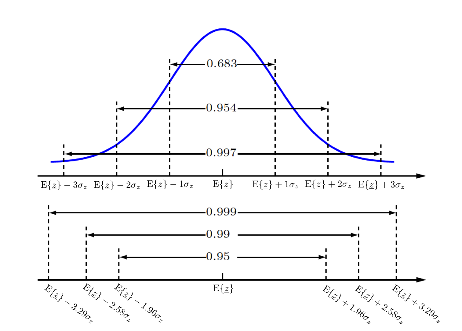
We have learned that for random variables with Gaussian/Normal distribution, we can define probabilistic intervals around their expectation. For example, the probability that random variable \(\underline{z}\) deviates less than \(2\sigma_z\) from its expectation value is given by: \[P(\underline{z}-\text{E}\{\underline{z}\} \in [-2\sigma_z,2\sigma_z]) = P(|\underline{z} - \text{E}\{\underline{z}\}| <2\sigma_z) = 0.954.\]

In other words,  there is a  95.4 percent chance that the random variable \(\underline{z}\) is inside the following interval \[ [\text{E}\{\underline{z}\}-2\sigma_z, \text{E}\{\underline{z}\}+2\sigma_z].\]

We will apply this concept to the estimators. Recall that if the observations have a normal distribution, the normality also holds for the linear estimators WLSE and BLUE. Note that, because these estimators are unbiased,  the expected value of these estimators equals the true (but unknown) value of the parameters of interest. However, the true value is never known, and so we cannot calculate the bounds of the aforementioned interval. For example, assume \(\underline{y}\) is normally distributed and we have a linear mathematical model as \(\text{E}\{\underline{y}\}=Ax\) and  \(\text{D}\{\underline{y}\}=Q_{yy}\).   Also for simplicity, let's assume that we have only one parameter in \(x\). The BLU estimator of \(x\) is then given as \[\hat{\underline{x}}=(A^TQ_{yy}^{-1}A)^{-1}A^TQ_{yy}^{-1}\underline{y}\] 

and its standard deviation can be computed as\[\sigma_{\hat{x}}=\sqrt{ (A^TQ_{yy}^{-1}A)^{-1}}\]

The estimator \(\hat{\underline{x}}\) is a random variable, and so we can apply the aforesaid interpretation of probabilistic intervals  about  \(\hat{\underline{x}}\). We can say:  the probability that the stochastic estimator \(\underline{\hat{x}}\) is within the following interval is 95.4% 

\[ [\text{E}\{\hat{\underline{x}}\}-2\sigma_{\hat{x}}, \text{E}\{\hat{\underline{x}}\}+2\sigma_{\hat{x}}].\] 

This is in fact the probabalistic interpretation of the estimator precesion, indicating that the probability that the estimator deviates from the true value is 95.4%.  

However,  if  we  want to calculate a certain interval as a probabalistic confidence interval, we cannot calculate the above interval \( [\text{E}\{\hat{\underline{x}}\}-2\sigma_{\hat{x}}, \text{E}\{\hat{\underline{x}}\}+2\sigma_{\hat{x}}]\), since \(\text{E}\{\hat{\underline{x}}\}=x\) is unknown.  Instead, in practice, the confidence interval is defined around the estimate \(\hat{x}\). For example, if \(x\) is a canal width for which we have an estimate of \(\hat{x}=10\)m with the estimator precision of 2 cm, then we write the 95.4% confidence  interval as

\[ [10-2\sigma_{\hat{x}}, 10+2\sigma_{\hat{x}}]=[9.96,~10.04] \text{m}.\] 

The rational behind this way of using confidence intervals (that is using an interval around the estimate, not around the expectation) is as follows:

The estimate \(\hat{x}\) is a realization of the random variable \(\hat{\underline{x}}\). As the estimator is unbiased  (\(\text{E}\{\hat{\underline{x}}\}=x\)), we have

\[P(\underline{\hat{x}} \in [\text{E}\{\hat{\underline{x}}\}-2\sigma_{\hat{x}},~~\text{E}\{\hat{\underline{x}}\}+2\sigma_{\hat{x}}])=\\    P(x-2\sigma_{\hat{x}}  < \underline{\hat{x}} < x+2\sigma_{\hat{x}})=0.954\]

If we subtract  \(x\)  and \(\underline{\hat{x}}\) from  all sides of above inequality, and multiply them by -1 we get

\[P(x-2\sigma_{\hat{x}}  < \underline{\hat{x}} < x+2\sigma_{\hat{x}})=\\P(\underline{\hat{x}}-2\sigma_{\hat{x}}  < x < \underline{\hat{x}}+2\sigma_{\hat{x}})=\\P(x \in [\underline{\hat{x}}-2\sigma_{\hat{x}},~~\underline{\hat{x}}+2\sigma_{\hat{x}}]) =0.954\]

Now we have a new stochastic interval \([\underline{\hat{x}}-2\sigma_{\hat{x}},~~\underline{\hat{x}}+2\sigma_{\hat{x}}]\) . It is stochastic because the estimator \(\underline{\hat{x}}\) is random. Let's call this interval \(\underline{S}\) (that is \(\underline{S}=[\underline{\hat{x}}-2\sigma_{\hat{x}},~~\underline{\hat{x}}+2\sigma_{\hat{x}}]\)).  If we now change the   \(\underline{\hat{x}}\) with the estimate \(\hat{x}\), we get  a realization of this stochastic interval   \[S=[\hat{x}-2\sigma_{\hat{x}},~~\hat{x}+2\sigma_{\hat{x}}].\]

Note the difference between \(S\) and  \(\underline{S}\). The realization interval \(S\) is the one that we use in practice as an confidence interval. But, in fact, it is just a realization of the stochastic confidence interval \(\underline{S}\).  The layman interpretation (which is commonly used in practice) of the confidence interval is that there is a low probability (in this case 100-95.4%) that the true unknown value \(x\) will be outside \(S\). The precise and exact meaning of the confidence interval, however, is that we have low probability (in this case 100-95.4%) that the stochastic interval \(\underline{S}\) does not cover the true parameter \(x\). That is, if the observation experiment were to be repeated many times and if the interval \(S\) were obtained for each case, then the relative frequency of those intervals that cover the true but unknown \(x\) would approach to 100-95%.  

Some important intervals for normal distribution

It is helpful to learn and remember some important probabilistic intervals of Gaussian/Normal distributions.  The figure below may help to memorize these probabilities and their corresponding intervals.