In the previous video, we learned about the so-called overall model test (OMT) that can be used to detect whether an error is present in the mathematical model or not. The  OMT test statistic is given by:

\[ \underline{T} = \underline{\hat{e}}^T Q_{yy}^{-1} \underline{\hat{e}}.\]

If the observations are normally distributed, it can be shown that the test statistic \(\underline{T}\) follows the central \(\chi^2\)-distribution (chi-square) with \(m-n\) degrees of freedom (where \(m\) is the number of observations, and \(n\) is the number of unknowns) :

\[\underline{T}\sim \chi^2(m-n,0).\]

Note that the \(\chi^2\)-distribution is defined for degrees of freedom equal to one or larger. So,  in case of no redundancy (i.e., \(m=n\)), the degrees of freedom is zero,  and the test is not applicable.  Knowing the distribution, it is possible to evaluate the probability that \(\underline{T}\) is larger than a certain value. The idea is then to choose a small probability (see the plot below), called \(\alpha\) and to find the corresponding value \(K\) such that:

\[P(\underline{T}>K) = \alpha\]

If we find a \(T\) that is larger than \(K\), the OMT is rejected, meaning it is likely that there is an error in the assumed mathematical model, since it is unlikely that \(T\) is larger than \(K\).

The parameter \(\alpha\) is called the level of significance, and it is usually chosen to be a small number (for example 0.05 or 0.001, depending on the application).   In fact, the level of significance is the probability that the overall model test is mistakenly or falsely rejected.  Note that, by choosing a smaller \(\alpha\), although the chance of false-rejection of the OMT is reduced, the chance of its false-acceptance increases.  So there is a trade-off between these two probabilities.    

After choosing the level of significance, the threshold \(K\) (or the critical value) corresponding to the chosen \(\alpha\)  can be obtained from the  \(\chi^2\) distribution function. In the following, you find more information how to compute the critical value for a chosen \(\alpha\). 

Computing the critical value in Matlab

In Matlab, you can use the function 'chi2inv' to define the critical value.  For example for \(\alpha=0.05\) and \(m-n=10\) , you can use  

chi2inv(1-0.05,10) which gives 18.307. 

Computing the critical value from the \(\chi^2\) table 

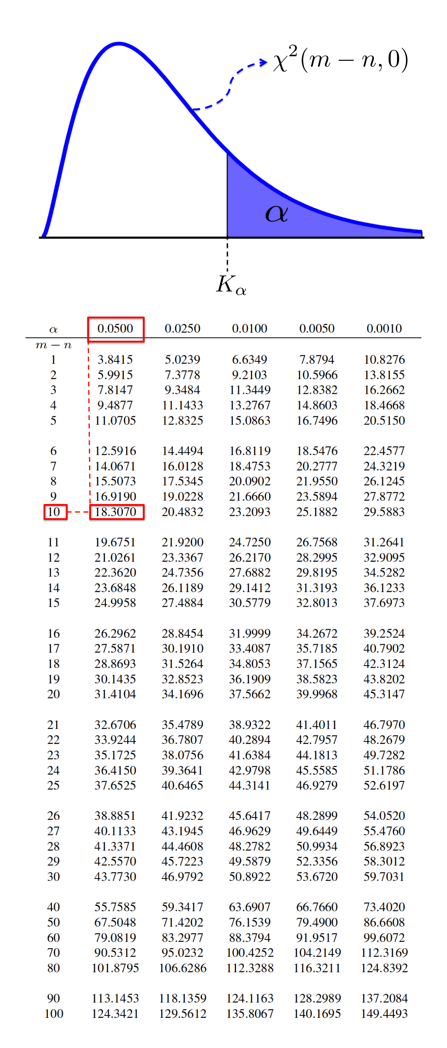
The table below shows the critical value \(K_\alpha\) of a random variable with a \(\chi^2(m-n,0)\)-distribution for some \(\alpha\) values and different degrees of freedom. 

As an example, if \(\alpha=0.05\) and \(m-n=10\), the critical value will be  \(K_{0.05}=18.307\) (For this example, the \(\alpha=0.05\), \(m-n=10\), and \(K_{0.05}\) have been highlighted in the following table with the red boxes).