


Population model
Course subject(s)
2. Improving the model
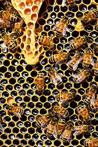
Honey Bee Honeycomb Queen Cup CC0
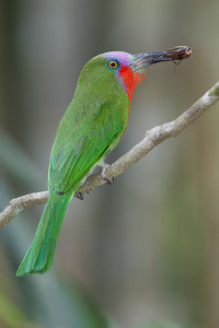
Red-bearded Bee-eater by J.J. Harrison CC BY-SA 3.0
interacting populations
Choose your own set of populations: animals, plants, bacteria… and model the size of the populations. One population might feed on the other, as with the gouramis and rainbowfish we use in the course in Module 3, but you can also choose two populations that compete for the same resources, such as rabbits and deer competing for the same grass. A third option is that the two species benefit from each other such as cleaner fishes and groupers.
Population model
The number of members in the first population is called u(t) and the number of members of the second population v(t).
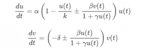
The parameters α,k,β,γ, and δ you will have to choose appropriately, as well as the signs some of the terms.
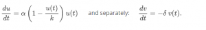
Simplified population model
After Module 3, you will let the populations interact, but for now, investigate the case of no interaction: β=0. For example, how does the antilope population grow when there are no lions, and how would the lion population fare, if there were no antilopes? So start with:
Tasks for the project in Module 2
-
- Decide on what two populations you want to model.
- Decide on a unit for the time t.
- Decide on units for u and v. If you are modelling the ants and anteaters in a large area, maybe units of 1000 ants are easier to work with. If it is grass and cows you are modelling, the unit of grass could be in kilograms per km2.
- With the units for u and v and the differential equations, you can determine the units for α, k, and δ.
- Try to find quantitative information on both populations. How large is a typical population, how old do they get, how many young do they raise, etc. If you cannot find that information, make an educated guess. Do not forget to write down where you found the information!
- Draw a phase line for v. Solve the equation for v analytically.
- Choose a value for δ such that the solution v(t) develops in a realistic way, not too fast, not too slow. You might not have enough information for a very precise value, so make a reasonable guess.
- Draw a phase line for u. Which of the equilibrium points are stable? Sketch also a direction field.
- Set the value of k to an appropriate value, such that the equilibrium values for u are appropriate. Again, you might not have enough information, so make a guess.
- You can try to give α a value, by considering the growth of the u‘s for a very small population, like we did for the rainbowfish. Some of you may have learned elsewhere the techniques to solve the differential equation for u analytically, and then you can use the analytical solution to adjust the value of α to fit your population u. You can also wait until the end of this module, when you will be able to approximate the solutions numerically.
Throughout, do communicate well with your teammate, so you make the different choices together. Document every result and decision in your logbook. That will help in the communication between you two, and when you are writing the report later on, you can find all your previous results easily.
After the pages for the other problems, you will find a page for questions you might have about the project.

Mathematical Modeling Basics by TU Delft OpenCourseWare is licensed under a Creative Commons Attribution-NonCommercial-ShareAlike 4.0 International License.
Based on a work at https://online-learning.tudelft.nl/courses/mathematical-modeling-basics/.