RELATIVE FREQUENCY OR EMPIRICAL PROBABILITY

The relative frequency or empirical probability is the ratio of the number of outcomes of a certain event and the total number of outcomes. 

Example: number of times \(n_i\) that a measurement \(\underline{y}\) was in a certain interval \([y_i, y_i +dy]\) divided by total number of measurements \(N \) is the relative frequency or empirical probability that the measurement is in that interval.

Notation: \( P \left(\underline{y} \in [y_i, y_i +dy]\right) = \dfrac{n_i}{N} \)

HISTOGRAM (RELATIVE FREQUENCIES)

The figure below shows a histogram with the relative frequencies that random variable \(\underline{y}\) is in the corresponding intervals; the range of values that \(\underline{y}\) can take is divided in intervals of equal width. As such, the height of each bar equals the empirical probability that the random variable is in the corresponding interval. The histogram shows the frequency distribution of the random variable.

HISTOGRAM (EMPIRICAL DENSITIES)

Instead of the relative frequencies, we can also make an histogram with the empirical density distribution. The empirical density is defined as \[f _{\underline{y}}(y_i) = \frac{ P (\underline{y} \in [y_i, y_i +dy]) }{dy}, \]

i.e., it is equal to the empirical probability divided by the interval length, or bin width.

[note the similarity with volumetric mass density being equal to mass divided by volume]

The advantage is that the empirical densities are insensitive to changes in the bin width \(dy\), in contrast to the relative frequencies, since a smaller bin width results in a smaller relative frequency.

The figure below shows a histogram with empirical densities for the same example as in previous figure. Note that the empirical probability is now equal to the area of a bar.

The probability that you are in a certain interval \( [y_j, y_m] \) with \(y_m = y_j + k\cdot dy \) (i.e. the interval has a length of \(k\) times \(dy\)), can be computed as

\[ P (\underline{y} \in [y_j, y_m])   =\sum_{i=j}^{j+k-1} f _{\underline{y}}(y_i) dy \]

It is the total area of the \(k\) bars of the histogram, as can be seen in the figure.

PROBABILITY DENSITY FUNCTION

A probability density function (PDF) is the continuous version of the histogram with densities (you can see this by imagining infinitesimal small bin widths); it specifies how the probability density is distributed over the range of values that a random variable can take. The figure below shows an example of an histogram and the corresponding continuous PDF.

The PDF of a random variable is often described by a certain analytical function. A large number of such statistical distribution functions has been defined, well-known examples are for example the uniform distribution and the normal distribution.

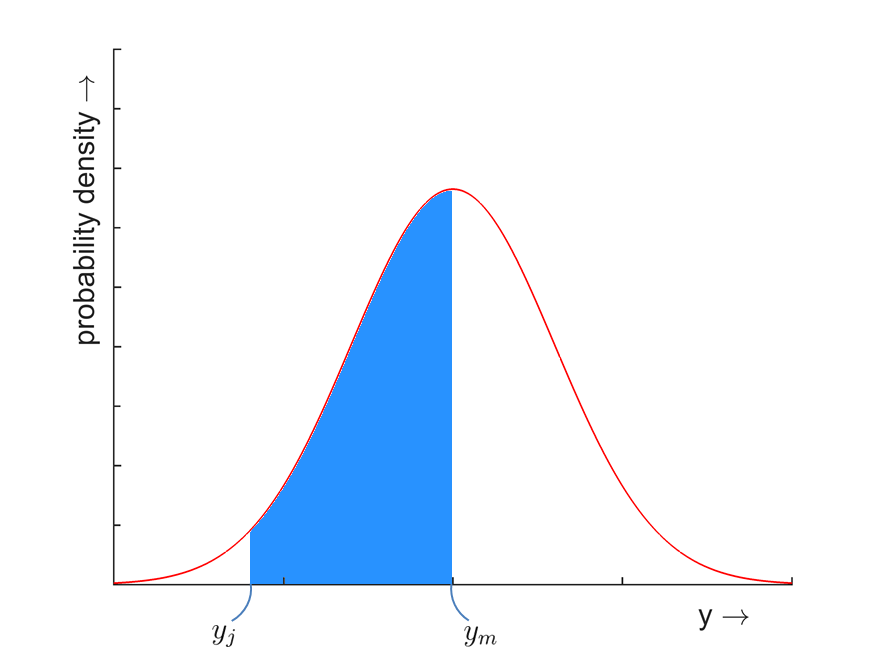
Similarly as with the histogram, the probability that a random variable takes a value in a certain interval \( [y_j, y_m] \) is equal to the area below the function, see figure below. It can be calculated by taking the integral over the interval: 

\[ P (\underline{y} \in [y_j, y_m])   =\int_{y_j}^{ y_m } f _{\underline{y}}(y) dy \]

Two important properties of the PDF are that \(f_{\underline{y}}(y) >0\), \(\forall y \) and \( \int_{-\infty}^{ \infty } f _{\underline{y}}(y) dy = 1 \).