Solar Cell Performance
Course subject(s)
3. Solar Cell Operation, Performance and Design Rules
In this video Prof. Arno Smets takes the perfect solar cell and derives the open circuit voltage generated when the solar cell is not connected to anything. He then derives the current generated when the cell is short circuited, and uses these two parameters to derive the power curve of the cell.
You will find the chapter associated to the lecture below the videos.
Fill Factor and Open-Circuit Voltage
The fill factor \(FF\) is defined as:
\(FF = \frac{J_{mp}*V_{mp}}{J_{sc}*V_{oc}}\tag{1} \)
where:
- \(J_{mp}\): current density at maximum power point
- \(V_{mp}\): voltage at maximum power point
- \(J_{sc}\): short-circuit current density
- \(V_{oc}\): open-circuit voltage
The maximum power produced by a solar cell occurs at the point where:
\( \frac{dP}{dV}=0 \) or in other words \( \frac{d}{dV}[J(V)*V]=0\) \( \tag{2}\)
Recall also from video block 3.1 10:03 that: \( J(V)= J_{ph}- J_o[exp(\frac{q*V}{n*k_B*T}) -1] \tag{3}\) where:
- \(k_B\): Boltzmann constant
- \(q\): elementary charge
- \(n\): ideality factor, which for this course is considered as 1
- \(T\): operating temperature
Therefore we can write that: \( \frac {d}{dV} \Big\{\big[J_{ph}- J_o(exp(\frac{q*V}{n*k_B*T}) -1)\big]*V\Big\} \Bigg|_{V=V_{mp}} =0 \tag{4} \)
Let \( \alpha=\frac{q}{n*k_B*T} \)
The above equation can be written as:
\( \frac {d}{dV} \Big\{\big[J_{ph}- J_o(exp(\alpha*V)-1)\big]*V\Big\} \Bigg|_{V=V_{mp}} =0 \tag{5}\)
Working out equation \((5)\) we can derive the relationship: \( \frac {J_{ph}}{J_o}+1=exp(\alpha*V_{mp})*(1+\alpha* V_{mp}) \tag{6}\)
However the \(V_{oc} \) is: \( V_{oc}=\frac {n*k*T}{q}*ln(\frac {J_{ph}}{J_o}+1) \tag{7}\)
which by replacing the term \( \frac {n*k_B*T}{q} \) becomes: \( V_{oc}=\frac {1}{\alpha}*ln(\frac {J_{ph}}{J_o}+1) \tag{8} \)
Taking the natural logarithm at both sides of equation \((6)\) and using \((8)\), we can derive: \( V_{mp}=V_{oc}-\frac {1}{\alpha}*ln(1+\alpha*V_{mp}) \tag{9} \)
Equation \((9)\) does not have an analytical solution. That means that we cannot solve \((9)\) for \( V_{mp} \).
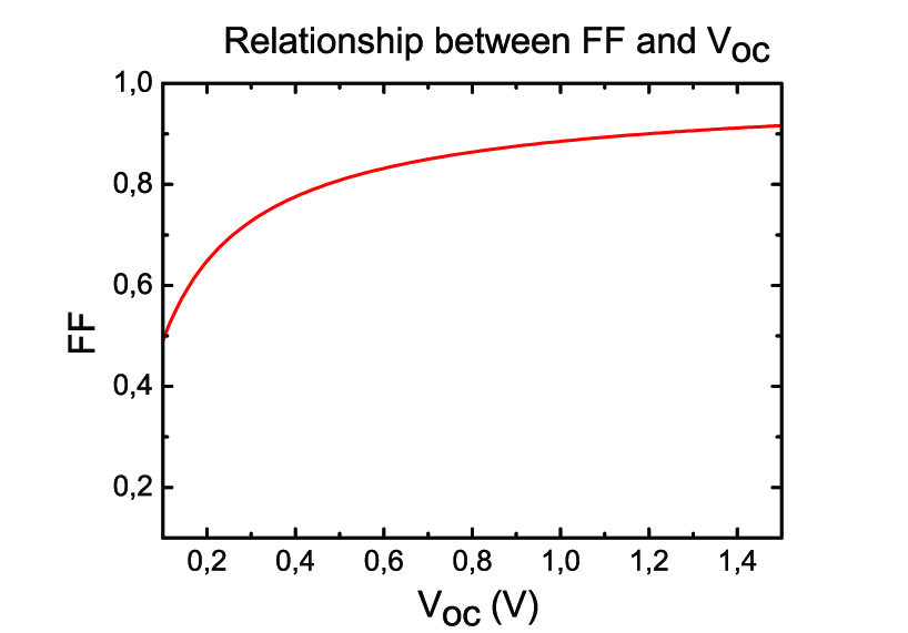
If we replace equation \((9)\) into equation \((1)\), we also notice that we cannot derive an analytical solution for \(FF\) and \(V_{oc}\).
An empirical relationship of \( FF \) and \(V_{oc}\) is the following: \( FF= \frac {{ \alpha}*V_{oc}-ln( {\alpha}*V_{oc}+0.72)}{{\alpha}*V_{oc}+1} \tag{10}\)
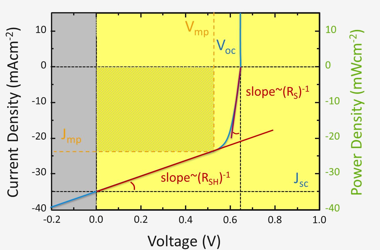
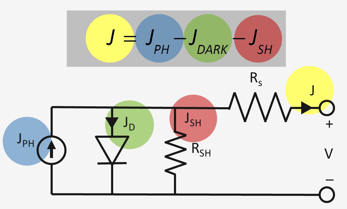
In the figure on the right the J-V curve of a non-ideal p-n junction is shown.
We are going to show that a fairly good estimation of the series resistance \(R_s\) can be made by finding the slope \( dJ/dV \) at the open-circuit voltage point \(V_{oc}\). Similarly we are going to show that the shunt resistance \(R_{sh}\) can be estimated from the slope \( dJ/dV \) at the short-circuit point \(J_{sc}\).